Configurations and Robot Transformations

Configuration, State, and Degrees of Freedom

Configuration and C-Space

The first question to answer in robotics is, simply, where is the robot?.
A proper complete answer would require knowing position of every single point in the robot with respect to some global frame. This complete specification is called the robot's configuration.

Configuration of a robot specifies the position of every point of the robot

A configuration, denoted by $q$ , is a set of parameters that uniquely defines the robot's state. The set of all possible configurations a robot can achieve is its configuration space, or C-space.
The C-space is a crazy concept because it transforms the complex geometric problem of a robot moving among obstacles in the physical workspace into a simpler problem of a single point moving in this higher-dimensional C-space. Configurations where the robot does not collide with obstacles are part of the collision-free C-space.

Degrees of Freedom (DOF)

The number of degrees of freedom (DOF) is the minimum number of independent parameters needed to completely specify the robot's configuration.
This means the DOF is also the dimension of the robot's C-space.

A point in a 2D plane has 2 DOF, described by $(x, y)$ .
A rigid body in a 2D plane requires three parameters: its position $(x, y)$ and its orientation $θ$ . It therefore has 3 DOF.
A rigid body in 3D space requires six parameters: its position $(x, y, z)$ and its orientation, which can be described by three angles (e.g., roll, pitch, yaw). It has 6 DOF.

We can develop an intuition for this by considering the constraints on a rigid body. In 2D, once we fix the position of a point A (2 DOF), a second point B is constrained to lie on a circle around A (1 more DOF). Any other point C is then fully determined by its distances to A and B. The total is $2 + 1 = 3$ DOF. In 3D, the circles become spheres, leading to $3 + 2 + 1 = 6$ DOF.

Robot Joints

Robots are typically composed of rigid bodies called links connected by joints. Joints introduce constraints and reduce the overall DOF of the system.
Pasted image 20250921022014.png

Pasted image 20250921021902.png

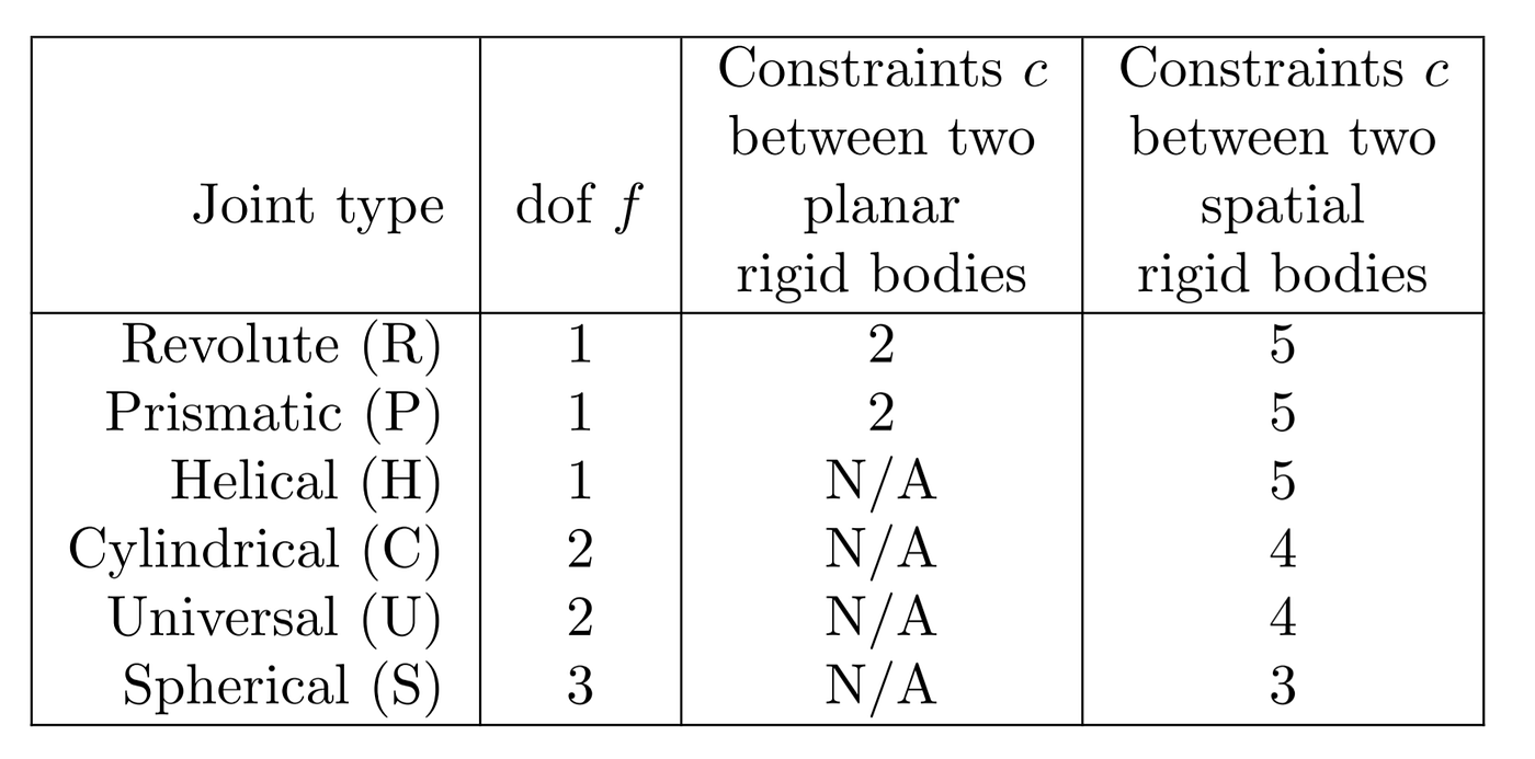
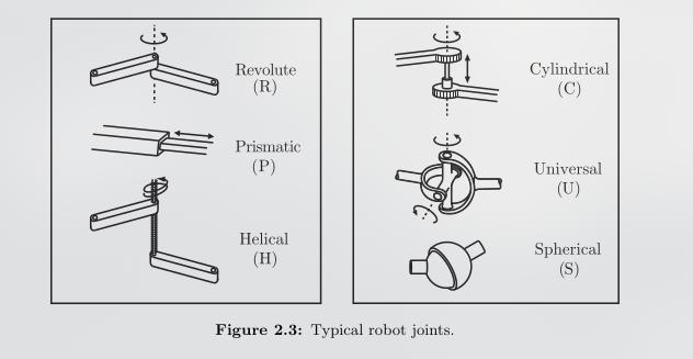
Image taken from Modern Robotics: Mechanics, Planning, and Control

Grübler's Formula

To calculate the DOF of a mechanism, we can use Grübler's Formula. This formula is based on the principle of subtracting the constraints imposed by joints from the total possible freedoms of the links.

D O F = m (N - 1 - J) + \sum_{i = 1}^{J} f_{i}

where:

$m$ is the DOF of a single rigid body in the workspace ( $m = 3$ for planar mechanisms, $m = 6$ for spatial mechanisms).
$N$ is the total number of links, including the fixed base (ground).
$J$ is the total number of joints.
$f_{i}$ is the number of freedoms provided by joint $i$ .

Example: A 3R Planar Arm
For a planar arm with three revolute joints connected in a series to a base:

It's a planar mechanism, so $m = 3$ .
There are 3 moving links and 1 ground link, so $N = 4$ .
There are 3 revolute joints, so $J = 3$ .
Each planar revolute joint has 1 DOF, so $f_{i} = 1$ for all three joints.

Plugging this into the formula:

D O F = 3 (4 - 1 - 3) + (1 + 1 + 1) = 3 (0) + 3 = 3

This confirms our intuition that the arm has 3 degrees of freedom.

Important Note: Grübler's formula is only valid if all joint constraints are independent. For some mechanisms with redundant constraints, it may yield an incorrect result.

Rigid Body Transformations in 2D

To describe a robot's configuration mathematically, we move from the notions of Euclidean geometry to the algebraic framework of Cartesian geometry. These are there in Co-ordinate-Transforms some what.

Coordinate Frames and Rotation

We attach coordinate frames to objects of interest.
A point $P$ can be represented as a vector from the origin of its frame, for example, $p = p_{x} \hat{x} + p_{y} \hat{y}$ . By convention, we use right-handed coordinate frames.

To describe a robot's motion, we need to relate points described in a local body frame ${B}$ to a global world frame ${W}$ . If frame ${B}$ is rotated by an angle $θ$ with respect to ${W}$ , we can find the coordinates of a point $p$ in the world frame, $p_{W}$ , from its coordinates in the body frame, $p_{B}$ .

The derivation proceeds as follows:

The basis vectors of ${B}$ in terms of ${W}$ using trigonometry:

{\hat{x}}_{B} = \cos θ {\hat{x}}_{W} + \sin θ {\hat{y}}_{W}

{\hat{y}}_{B} = - \sin θ {\hat{x}}_{W} + \cos θ {\hat{y}}_{W}

A point vector in the body frame is $p_{B} = p_{x B} {\hat{x}}_{B} + p_{y B} {\hat{y}}_{B}$ . Substitute the expressions from step 1 to find the same point vector relative to the world frame, $p_{W}$ :

p_{W} = p_{x B} (\cos θ {\hat{x}}_{W} + \sin θ {\hat{y}}_{W}) + p_{y B} (- \sin θ {\hat{x}}_{W} + \cos θ {\hat{y}}_{W})

Group the ${\hat{x}}_{W}$ and ${\hat{y}}_{W}$ terms:

p_{W} = (p_{x B} \cos θ - p_{y B} \sin θ) {\hat{x}}_{W} + (p_{x B} \sin θ + p_{y B} \cos θ) {\hat{y}}_{W}

This can be written in matrix form, which gives us the 2D rotation matrix:

[\begin{matrix} p_{x W} \\ p_{y W} \end{matrix}] = [\begin{matrix} \cos θ & - \sin θ \\ \sin θ & \cos θ \end{matrix}] [\begin{matrix} p_{x B} \\ p_{y B} \end{matrix}]

This relationship is compactly written as $p_{W} = R_{W B} p_{B}$ . The rotation matrix $R_{W B}$ transforms the coordinates of a point from frame ${B}$ to frame ${W}$ . This is very important distinction to make, the rotation matrix transforms the coordinates of a point from one frame to another, but if you apply the same rotation matrix to the basis vectors of the frame, it will give you the basis vectors of the other frame in the original frame's coordinates.

The Special Orthogonal Group $S O (2)$

Rotation matrices have several important properties:

They are orthogonal, meaning $R^{T} R = I$ . Therefore $R^{- 1} = R^{T}$
Their columns are mutually orthogonal unit vectors.
Their determinant is always $+ 1$ . A rotation preserves the length of vectors and the "handedness" of the coordinate system. (_Note: Not related to SO(2) but when we have determinant -1, it represents a reflection.)

The set of all $2 \times 2$ matrices that satisfy these properties forms the Special Orthogonal Group of dimension 2, denoted $S O (2)$ .

Homogeneous Transformations and $S E (2)$

When a frame is both rotated by $R$ and translated by a vector $t$ , the transformation is $p_{W} = R_{W B} p_{B} + t_{W B}$ . This mixes matrix multiplication and vector addition, which is annoying. We can combine them into a single matrix multiplication using homogeneous coordinates. We augment our vectors and matrices:

A 2D point $p = (p_{x}, p_{y})$ becomes a 3D vector $\tilde{p} = (p_{x}, p_{y}, 1)^{T}$ .
The transformation becomes a $3 \times 3$ matrix $T = [\begin{matrix} R & t \\ 0 & 1 \end{matrix}]$ .

Now, the transformation is a single, clean multiplication: ${\tilde{p}}_{W} = T_{W B} {\tilde{p}}_{B}$ .

[\begin{matrix} p_{x W} \\ p_{y W} \\ 1 \end{matrix}] = [\begin{matrix} \cos θ & - \sin θ & t_{x} \\ \sin θ & \cos θ & t_{y} \\ 0 & 0 & 1 \end{matrix}] [\begin{matrix} p_{x B} \\ p_{y B} \\ 1 \end{matrix}]

These $3 \times 3$ transformation matrices form the Special Euclidean Group of dimension 2, or $S E (2)$ . An advantage is that composing transformations is as simple as matrix multiplication: $T_{W A} = T_{W B} T_{B A}$ .
(That's because it's a property of SE(2) that the composition of two transformations is another transformation in SE(2).)

The fundamental insight is that the columns of a rotation matrix $R_{W B}$ are the basis vectors of the "new" frame ${B}$ expressed in the coordinates of the "old" frame ${W}$ . This allows us to transform the coordinates of any point from frame ${B}$ to frame ${W}$ via matrix multiplication:

p_{W} = R_{W B} p_{B}

When we need to account for both rotation and translation, we use homogeneous coordinates. This combines the rotation matrix $R$ and a translation vector $t$ into a single transformation matrix $T$ , allowing us to represent a full rigid body motion with a single matrix multiplication:

[\begin{matrix} p_{W} \\ 1 \end{matrix}] = [\begin{matrix} R & t \\ 0 & 1 \end{matrix}] [\begin{matrix} p_{B} \\ 1 \end{matrix}]

Example

A point $p_{B} = (2, 3, 5)$ is defined on a body ${B}$ , which is initially coincident with the world frame ${W}$ . The body is first rotated about its own Z-axis by $π / 2$ , then rotated about its new, local X-axis by $π / 2$ . Finally, it is translated by $t = (8, 1, 0)$ with respect to the world frame. Find the final coordinates of the point in the world frame, $p_{W}$ .

The first rotation is by $θ_{1} = π / 2$ about the Z-axis.

R_{1} = R_{z} (π / 2) = [\begin{matrix} \cos (π / 2) & - \sin (π / 2) & 0 \\ \sin (π / 2) & \cos (π / 2) & 0 \\ 0 & 0 & 1 \end{matrix}] = [\begin{matrix} 0 & - 1 & 0 \\ 1 & 0 & 0 \\ 0 & 0 & 1 \end{matrix}]

The second rotation is by $θ_{2} = π / 2$ about the new local X-axis.

R_{2} = R_{x} (π / 2) = [\begin{matrix} 1 & 0 & 0 \\ 0 & \cos (π / 2) & - \sin (π / 2) \\ 0 & \sin (π / 2) & \cos (π / 2) \end{matrix}] = [\begin{matrix} 1 & 0 & 0 \\ 0 & 0 & - 1 \\ 0 & 1 & 0 \end{matrix}]

To find the final orientation of the body, we post-multiply the first rotation by the second.

R_{W B} = R_{1} R_{2} = R_{z} (π / 2) R_{x} (π / 2) = [\begin{matrix} 0 & - 1 & 0 \\ 1 & 0 & 0 \\ 0 & 0 & 1 \end{matrix}] [\begin{matrix} 1 & 0 & 0 \\ 0 & 0 & - 1 \\ 0 & 1 & 0 \end{matrix}] = [\begin{matrix} 0 & 0 & 1 \\ 1 & 0 & 0 \\ 0 & 1 & 0 \end{matrix}]

Now we can find the final coordinates $p_{W}$ by applying the combined rotation and the final translation to the original point $p_{B}$ .

p_{W} = R_{W B} p_{B} + t

p_{W} = [\begin{matrix} 0 & 0 & 1 \\ 1 & 0 & 0 \\ 0 & 1 & 0 \end{matrix}] [\begin{matrix} 2 \\ 3 \\ 5 \end{matrix}] + [\begin{matrix} 8 \\ 1 \\ 0 \end{matrix}] = [\begin{matrix} (0 \cdot 2 + 0 \cdot 3 + 1 \cdot 5) \\ (1 \cdot 2 + 0 \cdot 3 + 0 \cdot 5) \\ (0 \cdot 2 + 1 \cdot 3 + 0 \cdot 5) \end{matrix}] + [\begin{matrix} 8 \\ 1 \\ 0 \end{matrix}]

p_{W} = [\begin{matrix} 5 \\ 2 \\ 3 \end{matrix}] + [\begin{matrix} 8 \\ 1 \\ 0 \end{matrix}] = [\begin{matrix} 13 \\ 3 \\ 3 \end{matrix}]

The final coordinates of the point are $(13, 3, 3)$ .

Singularities in Orientation: Gimbal Lock

While representing orientation with a sequence of three rotations (Euler angles) is intuitive, it suffers from a critical problem known as gimbal lock. This is a singularity where the alignment of two rotation axes causes the loss of one degree of rotational freedom. I cover this in more detail in my EULER ANGLES note.

Let's examine the mathematical reason for this. Consider a ZYX roll-pitch-yaw convention. The final rotation is $R = R_{z} (y) R_{y} (p) R_{x} (r)$ . If the pitch angle $p$ is set to $π / 2$ :

R_{y} (π / 2) = [\begin{matrix} 0 & 0 & 1 \\ 0 & 1 & 0 \\ - 1 & 0 & 0 \end{matrix}]

The full rotation becomes:

R = R_{z} (y) R_{y} (π / 2) R_{x} (r)

A useful property of rotation matrices states that $R_{y} (π / 2) R_{x} (r) = R_{z} (r) R_{y} (π / 2)$ . Substituting this in:

R = R_{z} (y) R_{z} (r) R_{y} (π / 2) = R_{z} (y + r) R_{y} (π / 2)

The final orientation now depends only on the sum of the yaw and roll angles, not their individual values. We can no longer distinguish between a yaw and a roll motion; the system has become degenerate and lost a degree of freedom.

Axis-Angle Representation

An alternative, non-singular way to represent orientation is the axis-angle form. Euler's rotation theorem states that any orientation in 3D space can be described as a single rotation by an angle $θ$ about a single unit axis $\hat{w}$ . This is often more intuitive than a sequence of three separate rotations.

Rodrigues' Formula Derivation

Rodrigues' formula provides a direct mapping from an axis $\hat{w}$ and angle $θ$ to the equivalent $3 \times 3$ rotation matrix $R (\hat{w}, θ)$ . The slides note this was a derivation on the board, so here are the steps.

Step 1: Decompose the Vector

We want to rotate a vector $v$ around the unit axis $\hat{w}$ . We can decompose $v$ into two components: one parallel to $\hat{w}$ and one perpendicular to $\hat{w}$ .

v = v_{| |} + v_{⊥}

The parallel component is the projection of $v$ onto $\hat{w}$ :

v_{| |} = (\hat{w} \cdot v) \hat{w}

The perpendicular component is what remains:

v_{⊥} = v - v_{| |} = v - (\hat{w} \cdot v) \hat{w}

Step 2: Rotate the Components

The rotation only affects the perpendicular component. The parallel component lies on the axis of rotation and is therefore unchanged.

v_{| |, r o t} = v_{| |}

The component $v_{⊥}$ rotates by angle $θ$ in the plane whose normal is $\hat{w}$ . The rotated vector, $v_{⊥, r o t}$ , can be described as a sum of a component along the original $v_{⊥}$ and a component along the vector orthogonal to both $\hat{w}$ and $v_{⊥}$ (which is given by $\hat{w} \times v$ ).

v_{⊥, r o t} = (\cos θ) v_{⊥} + (\sin θ) (\hat{w} \times v_{⊥})

Since $\hat{w}$ and $v_{| |}$ are parallel, their cross product is zero, meaning $\hat{w} \times v = \hat{w} \times (v_{| |} + v_{⊥}) = \hat{w} \times v_{⊥}$ . So we can write:

v_{⊥, r o t} = (\cos θ) v_{⊥} + (\sin θ) (\hat{w} \times v)

Step 3: Recombine and Simplify

The final rotated vector, $v_{r o t}$ , is the sum of the rotated components.

v_{r o t} = v_{| |, r o t} + v_{⊥, r o t} = v_{| |} + (\cos θ) v_{⊥} + (\sin θ) (\hat{w} \times v)

Substitute the expressions for $v_{| |}$ and $v_{⊥}$ :

v_{r o t} = (\hat{w} \cdot v) \hat{w} + \cos θ (v - (\hat{w} \cdot v) \hat{w}) + \sin θ (\hat{w} \times v)

Grouping terms for $v$ and $(\hat{w} \cdot v) \hat{w}$ :

v_{r o t} = v \cos θ + (\hat{w} \cdot v) \hat{w} (1 - \cos θ) + (\hat{w} \times v) \sin θ

This is the vector form of Rodrigues' formula.

Step 4: Convert to Matrix Form

To get the matrix $R$ such that $v_{r o t} = R v$ , we can represent the cross product as a matrix multiplication using the skew-symmetric matrix of $\hat{w}$ , denoted $[\hat{w}]$ :

[\hat{w}] v = \hat{w} \times v ⟹ [\hat{w}] = [\begin{matrix} 0 & - w_{z} & w_{y} \\ w_{z} & 0 & - w_{x} \\ - w_{y} & w_{x} & 0 \end{matrix}]

The term $(\hat{w} \cdot v) \hat{w}$ can be written as $(\hat{w} {\hat{w}}^{T}) v$ . Also, a useful identity is $[\hat{w}]^{2} = \hat{w} {\hat{w}}^{T} - I$ .
Substituting these into the vector formula gives the final matrix form of Rodrigues' formula:

R (\hat{w}, θ) = I \cos θ + (\hat{w} {\hat{w}}^{T}) (1 - \cos θ) + [\hat{w}] \sin θ

Using the identity for $[\hat{w}]^{2}$ , this is more commonly written as:

R (\hat{w}, θ) = I + \sin θ [\hat{w}] + (1 - \cos θ) [\hat{w}]^{2}