Generalized Linear Models

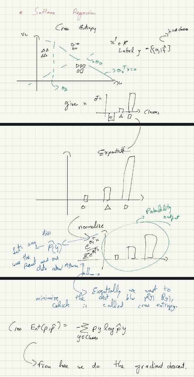
GLMs are here babby!!!.

We need to understand more about exponential family distributions before we get into GLMs.

p (y; η) = b (y) \exp (η^{T} T (y) - a (η))

Where all of the terms are:

$y$ is data.
$η$ is natural parameter.
$T (y)$ is called sufficient statistics.
$b (y)$ is base measure.
$a (η)$ is log-partition.

Quick observation tells us that these functions are only of certain parameters, so T(y) is a function only and only of y and not $η$ .

Some of the common exponential as these functions are:

Bernoulli:

\begin{aligned} p (y; ϕ) & = ϕ^{y} (1 - ϕ)^{1 - y} \\ = \exp (y \log ϕ + (1 - y) \log (1 - ϕ)) \\ = \exp ((\log (\frac{ϕ}{1 - ϕ})) y + \log (1 - ϕ)) \end{aligned}

η = \log (ϕ / (1 - ϕ))

T (y) = y

a (η) = - \log (1 - ϕ) = \log (1 + e^{η})

b (y) = 1

Gaussian with variance = 1:

σ^{2} = 1

p (y; μ) = \frac{1}{\sqrt{2 π}} \exp (- \frac{1}{2} y^{2}) \exp (μ y - \frac{1}{2} μ^{2})

η = μ

T (y) = y

a (η) = μ^{2} / 2 = η^{2} / 2

b (y) = (1 / \sqrt{2 π}) \exp (- y^{2} / 2)

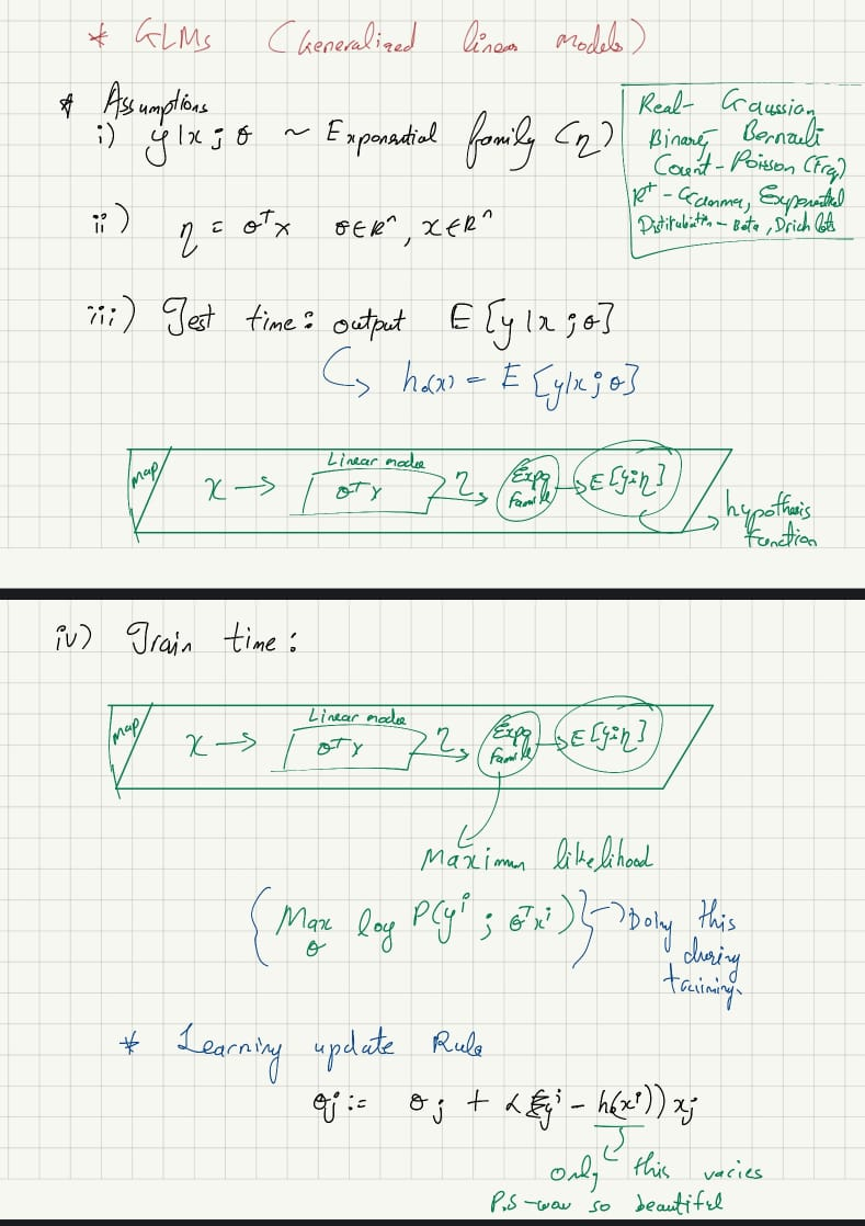
Overview of GLMs:

Pasted image 20240612115714.png
Pasted image 20240612115721.png

Softmax Regression:

In a broader case, we can have multiple classes instead of the binary classes above. It is natural to model it as a Multinomial distribution, which also belongs to the exponential family that can be derived from the Generalized Linear Model (GLM).

In multinomial, we can define $ϕ_{1}, ϕ_{2}, \dots, ϕ_{k - 1}$ to be the corresponding probabilities of $k - 1$ classes. We do not need all $k$ classes since the last one is determined once the previous $k - 1$ are set. So we can write $ϕ_{k} = 1 - \sum_{i = 1}^{k - 1} ϕ_{i}$ .

We first define $T (y) \in R^{k - 1}$ and :

T (1) = [\begin{matrix} 1 \\ 0 \\ ⋮ \\ 0 \end{matrix}], T (2) = [\begin{matrix} 0 \\ 1 \\ ⋮ \\ 0 \end{matrix}], \dots, T (k) = [\begin{matrix} 0 \\ 0 \\ ⋮ \\ 0 \end{matrix}]

Note that for $T (k)$ , we just have all zeros in the vector since the length of the vector is $k - 1$ . We let $T (y)_{i}$ define the $i$ -th element in the vector.

Now, we show the steps to derive the Multinomial distribution as an exponential family:

\begin{aligned} p (y; ϕ) & = ϕ_{1}^{[y = 1]} ϕ_{2}^{[y = 2]} \dots ϕ_{k}^{[y = k]} \\ = ϕ_{1}^{[y = 1]} ϕ_{2}^{[y = 2]} \dots ϕ_{k}^{1 - \sum_{i = 1}^{k - 1} [y = i]} \\ = ϕ_{1}^{T (y)_{1}} ϕ_{2}^{T (y)_{2}} \dots ϕ_{k}^{1 - \sum_{i = 1}^{k - 1} T (y)_{i}} \\ = \exp (T (y)_{1} \log (\frac{ϕ_{1}}{ϕ_{k}}) + T (y)_{2} \log (\frac{ϕ_{2}}{ϕ_{k}}) + \dots + T (y)_{k - 1} \log (\frac{ϕ_{k - 1}}{ϕ_{k}}) + \log (ϕ_{k})) \\ = b (y) \exp (η^{T} T (y) - a (η)) \end{aligned}

where

η = [\begin{matrix} \log (\frac{ϕ_{1}}{ϕ_{k}}) \\ \log (\frac{ϕ_{2}}{ϕ_{k}}) \\ ⋮ \\ \log (\frac{ϕ_{k - 1}}{ϕ_{k}}) \end{matrix}]

and

a (η) = - \log (ϕ_{k}), b (y) = 1.

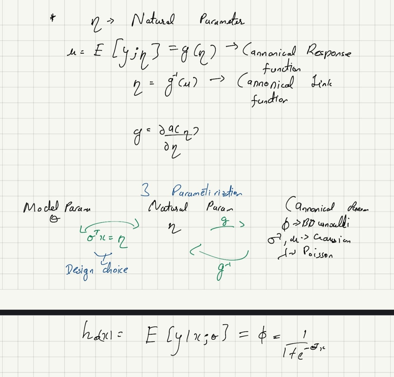
This formulates the multinomial distribution as an exponential family. We can now have the link function as:

η_{i} = \log (\frac{ϕ_{i}}{ϕ_{k}})

To get the response function, we need to invert the link function:

\begin{aligned} e^{η_{i}} & = \frac{ϕ_{i}}{ϕ_{k}} \\ ϕ_{k} e^{η_{i}} & = ϕ_{i} \\ ϕ_{k} \sum_{i = 1}^{k} e^{η_{i}} & = \sum_{i = 1}^{k} ϕ_{i} \end{aligned}

Then, we have the response function:

ϕ_{i} = \frac{e^{η_{i}}}{\sum_{j = 1}^{k} e^{η_{j}}}

This response function is called the softmax function.

From the assumption (3) in GLM, we know that $η_{i} = θ_{i}^{T} x$ for $i = 1, 2, \dots, k - 1$ and $θ_{i} \in R^{n + 1}$ is the parameter of our GLM model and $θ_{k}$ is just 0 so that $η_{k} = 0$ . Now, we have the model based on $x$ :

p (y = i | x; θ) = ϕ_{i} = \frac{e^{θ_{i}^{T} x}}{\sum_{j = 1}^{k} e^{θ_{j}^{T} x}}

This model is called softmax regression, which is a generalization of logistic regression. Thus, the hypothesis will be:

h_{θ} (x) = E [T (y) | x; θ] = [\begin{matrix} ϕ_{1} \\ ϕ_{2} \\ ⋮ \\ ϕ_{k - 1} \end{matrix}] = [\begin{matrix} \frac{e^{θ_{1}^{T} x}}{\sum_{j = 1}^{k} e^{θ_{j}^{T} x}} \\ \frac{e^{θ_{2}^{T} x}}{\sum_{j = 1}^{k} e^{θ_{j}^{T} x}} \\ ⋮ \\ \frac{e^{θ_{k - 1}^{T} x}}{\sum_{j = 1}^{k} e^{θ_{j}^{T} x}} \end{matrix}]

Now, we need to fit $θ$ such that we can maximize the log-likelihood. By definition, we can write it out:

L (θ) = \sum_{i = 1}^{m} \log (p (y^{(i)} | x^{(i)}; θ)) = \sum_{i = 1}^{m} \log (\prod_{l = 1}^{k} {(\frac{e^{θ_{l}^{T} x}}{\sum_{j = 1}^{k} e^{θ_{j}^{T} x}})}^{1 {y^{(i)} = l}})

We can use gradient descent or Newton’s method to find the maximum of it.

Note: Logistic regression is a binary case of softmax regression. The sigmoid function is a binary case of the softmax function.

Overview simplified:

Pasted image 20240612121923.png

GDA