Mapping and 3D Representations

Before starting anything, a lot is taken from the one and only Cyrll Stachniss lectures. Link to the lecture .

Point Clouds

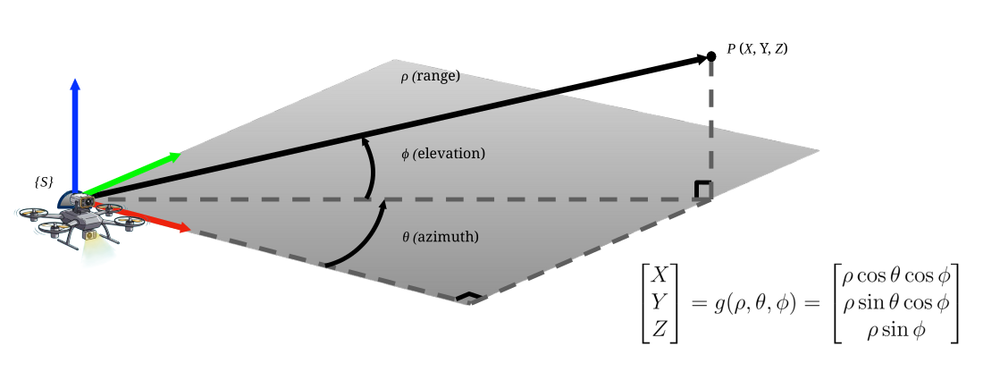
A point cloud is one of the most fundamental ways to represent a 3D environment. It is essentially a large collection of points where each point has an $(x, y, z)$ coordinate.

These points are often generated by sensors like LIDAR, which measures distance ( $ρ$ ), azimuth angle ( $θ$ ), and elevation angle ( $ϕ$ ). These raw spherical coordinates are then converted into Cartesian coordinates $(X, Y, Z)$ to form the point cloud using the following sensor model:

Pasted image 20250919121618.png

[\begin{matrix} X \\ Y \\ Z \end{matrix}] = g (ρ, θ, ϕ) = [\begin{matrix} ρ \cos (θ) \cos (ϕ) \\ ρ \sin (θ) \cos (ϕ) \\ ρ \sin (ϕ) \end{matrix}]

Pros:
- No data discretization is required, so the original measurement precision is maintained.
- The mapped area is not limited by a predefined grid size.
Cons:
- Memory usage can be unbounded as more points are added.
- There is no explicit representation of free or unknown space, only surfaces where the sensor light reflects are recoreded.

Operations on Point Clouds

The basic operations of translation and rotation can be combined. A common sequence to transform a point cloud $P_{s}$ from a source frame ${s}$ to a target frame ${s^{'}}$ is: 1) translate, 2) rotate, and 3) scale.

For each point $p_{s}$ in the cloud, the new point $p_{s^{'}}$ is given by:

p_{s^{'}} = S_{s^{'} s} R_{s^{'} s} (p_{s} - t_{s^{'} s})

Where:

$t_{s^{'} s}$ is the translation vector.
$R_{s^{'} s}$ is the rotation matrix.
$S_{s^{'} s}$ is a scaling matrix.

Feature Extraction from Point Clouds

A raw point cloud is just a collection of coordinates.
To make it useful, we often need to extract higher-level features from it, like planes, spheres, or cylinders. This process of identifying geometric primitives is a form of segmentation.

Point Cloud Accumulation

A single LIDAR scan only provides a point cloud from one perspective. To build a complete map, multiple point clouds taken from different robot poses must be combined into a single, global reference frame {G}. This process is called accumulation. ( Usually we take a defined global frame, or just the first frame )

If we have a point cloud $P_{L}$ measured in the local LIDAR frame {L}, and we know the pose (position and orientation) of the LIDAR frame with respect to the global frame, we can transform point cloud into global coordinates, $P_{G}$ . This is done using a homogeneous transformation matrix $_{L}^{G} T$ .

For each point $p_{i}$ in the local point cloud $P_{L}$ , the corresponding global point $p_{i}^{'}$ is calculated as:

p_{i}^{'} =_{L}^{G} T p_{i}

By applying this transformation to all points, we can merge multiple scans to create a dense, large-scale map of the environment.

Plane Fitting for Road Detection

A common task for an autonomous vehicle is to identify the road surface from a LIDAR point cloud. We can model the road as a simple plane and then fit this model to the point cloud data.

The equation of a plane in 3D is:

z = a + b x + c y

Our goal is to find the parameters $x = [a, b, c]^{T}$ that best fit the measured points. ( Think of this as a linear regression problem in 3D )

For a set of $n$ points $(x_{j}, y_{j}, z_{j})$ from the point cloud, we can define the measurement error for each point as the vertical distance between the measured $z_{j}$ and the value predicted by our plane model:

e_{j} = z_{p r e d i c t e d} - z_{m e a s u r e d} = (a + b x_{j} + c y_{j}) - z_{j}

We can stack all $n$ of these error equations into a single matrix form:

e = A x - b

Where:

e = [\begin{matrix} e_{1} \\ e_{2} \\ ⋮ \\ e_{n} \end{matrix}], A = [\begin{matrix} 1 & x_{1} & y_{1} \\ 1 & x_{2} & y_{2} \\ ⋮ & ⋮ & ⋮ \\ 1 & x_{n} & y_{n} \end{matrix}], x = [\begin{matrix} a \\ b \\ c \end{matrix}], b = [\begin{matrix} z_{1} \\ z_{2} \\ ⋮ \\ z_{n} \end{matrix}]

Now to find the best-fit parameters $\hat{x}$ , we use the method of least-squares to minimize the sum of the squared errors. The cost function is:

L_{L S} (x) = e^{T} e = (A x - b)^{T} (A x - b)

To find the minimum, we take the partial derivative with respect to $x$ and set it to zero:

\frac{\partial L_{L S} (x)}{\partial x} = 2 A^{T} A \hat{x} - 2 A^{T} b = 0

This gives us the normal equations:

A^{T} A \hat{x} = A^{T} b

We can then solve for the optimal parameters $\hat{x}$ by using an efficient numerical solver (ideally we use this in practice ) or by calculating the pseudo-inverse:

\hat{x} = (A^{T} A)^{- 1} A^{T} b

This gives us the parameters $[a, b, c]$ of the plane that best represents the road surface in the point cloud.

Voxel Grids

While point clouds are a direct representation of sensor data, they can be inefficient for tasks like collision checking.
Voxel grids address this by discretizing 3D space into a grid of volumetric elements, or voxels.

Pros:
- Volumetric representation of space.
- Constant access time.
- Allows probabilistic updates.
Cons:
- Memory requirements can be very high, as the entire volume of the map is allocated.
- The map's extent must be known beforehand.

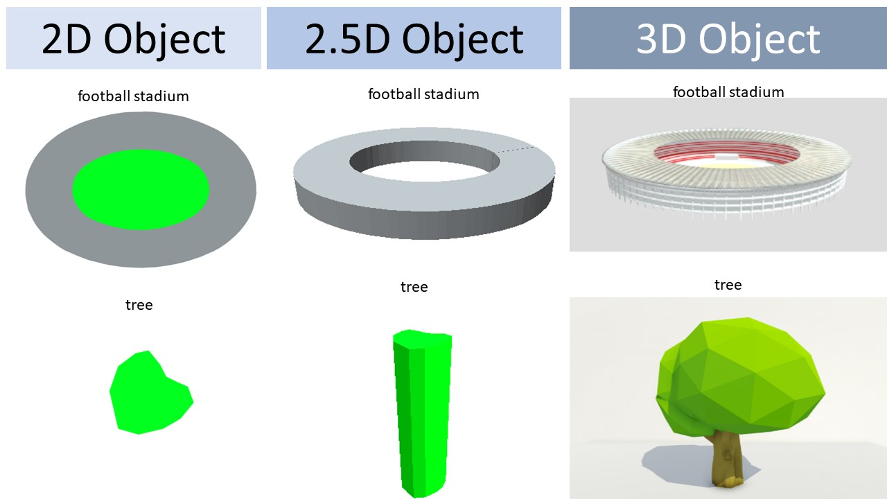
2.5D Maps / Height Maps

A common simplification of a full 3D voxel grid is a 2.5D map, often called a height map. Instead of storing a full 3D grid, a 2.5D map is a 2D grid where each cell stores a single height value, typically representing the highest point of an object within that cell's column.

Random Link: 2.5-D-Scene-Representation
A simple way to generate this is to average all the scan points that fall into a given (x,y) grid cell.

Pasted image 20250919145531.png

This representation is very memory efficient and provides constant-time access, but it's non-probabilistic and cannot distinguish between free and unknown space.

Elevation Maps

An elevation map is a more sophisticated, probabilistic version of a height map. Instead of just storing an average height, each cell stores a probabilistic estimate of the height, often updated using a Kalman filter. This allows the map to represent uncertainty, which typically increases with the measured distance from the sensor.

Pros:
- Memory efficient 2.5D representation.
- Provides a probabilistic estimate of height.
Cons:
- Cannot represent vertical objects or multiple levels (like a bridge over a road).

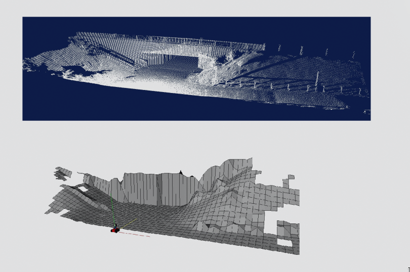
Multi-Level Surface (MLS) Maps

To overcome the single-level limitation of elevation maps, Multi-Level Surface (MLS) maps can be used. An MLS map allows each 2D cell to store multiple surface "patches". This enables the representation of complex vertical structures like bridges and underpasses.

Each patch in a cell consists of:

The height mean, $μ$
The height variance, $σ^{2}$
A depth value, $d$

TODO: Add more here, conversion from LIDAR to MLS .

Octrees (OctoMap)

While voxel grids are powerful, their memory usage is a significant drawback, especially in 3D where most cells are empty.
The Octree is a hierarchical data structure that efficiently addresses this problem by only allocating memory for volumes as needed.

An Octree works by recursively subdividing 3D space. A root node represents the entire volume. If this volume is not homogeneous (i.e., not entirely occupied, free, or unknown), it is subdivided into eight children nodes ("octants"), each representing a sub-volume. This process continues until a minimum voxel size is reached or a node's volume is homogeneous.

Pros:
- It is a full 3D model that is memory efficient.
- Can be updated probabilistically using a log-odds representation, just like occupancy grids.
- It is inherently multi-resolution, allowing for queries at different levels of detail.
- Open Source available here
Cons:
- The implementation IS tricky.

TODO: Probabilistic map updates, Kalman Filter pre-context and Bayes pre-context for adding more content.

Signed Distance Functions (SDF)

A Signed Distance Function (SDF) is way to represent geometry implicitly. An SDF is a function $f (p) : R^{3} \to R$ that, for any point $p$ in space, returns the shortest distance to a surface.

The sign of the function indicates whether the point is inside (negative) or outside (positive) the surface.
The surface itself is the set of all points where the function is zero, known as the zero level-set.

For example, the SDF for a sphere of radius $r$ centered at the origin is:

f (p) = | | p | | - r

A key property is that the gradient of the SDF, $\nabla f (p)$ , is a unit vector that always points in the direction of the closest point on the surface. This is extremely useful for optimization-based algorithms in motion planning and reconstruction.

Occupancy Grids

An occupancy grid is a specific type of voxel grid where each cell $m_{i}$ stores the probability $P (m_{i})$ that the corresponding region of space is occupied. This is powerful because it explicitly models uncertainty and distinguishes between occupied, free, and unknown space.

The map is updated sequentially using a Bayesian filter. Given a new measurement $z_{t}$ , we want to update the probability of a cell $m_{i}$ being occupied. Using Bayes' rule, the update is:

P (m_{i} | z_{1 : t}) = \frac{P (z_{t} | m_{i}, z_{1 : t - 1}) P (m_{i} | z_{1 : t - 1})}{P (z_{t} | z_{1 : t - 1})}

This can be computationally expensive. A more efficient way to handle this is to use the log-odds representation. The odds of a cell being occupied are $\frac{P (m_{i})}{1 - P (m_{i})}$ , and the log-odds are:

l (m_{i}) = \log \frac{P (m_{i})}{1 - P (m_{i})}

The update then becomes a simple addition:

l_{t} (m_{i}) = l_{t - 1} (m_{i}) + l_{i n v e r s e_s e n s o r_m o d e l}

Here, $l_{i n v e r s e_s e n s o r_m o d e l}$ is a pre-calculated log-odds value based on the sensor model. A positive value increases the belief of occupancy (e.g., for the cell where the beam ends), and a negative value increases the belief of the cell being free (for cells the beam passes through). This avoids costly multiplications and makes the map update very fast.

Probabilistic Map Update (Deeper Dive)

The occupancy of each voxel in a grid, $m_{i}$ , is updated using a recursive binary Bayes filter. The belief $B e l (m_{i})$ is updated based on a new measurement $z_{t}$ .

The update rule in log-odds form is efficient and avoids numerical instability near probabilities of 0 or 1.

l_{t} (m_{i}) = l_{t - 1} (m_{i}) + l_{i n v e r s e_s e n s o r_m o d e l}

Clamping Policy: To prevent probabilities from becoming permanently fixed at 0 or 1 (making them impossible to update later), a clamping policy is often used. This keeps the log-odds value within a certain range, for example, $l (m_{i}) \in [l_{m i n}, l_{m a x}]$ . This ensures the map can adapt to dynamic changes in the environment.
Multi-Resolution Queries: In hierarchical structures like OctoMaps, the belief of a parent node (a larger voxel) can be quickly determined from its children. A common approach is to set the parent's occupancy to the maximum occupancy value of its eight children. This allows for fast queries at different levels of detail.
$B e l (n_{p a r e n t}) = max_{i = 1. . .8} B e l (n_{c h i l d_{i}})$