Hierarchical Clustering

Builds a tree-based hierarchy of clusters, which is often visualized using a diagram called a dendrogram.

Types of Hierarchical Clustering

• Agglomerative Clustering (Bottom-Up): The algorithm starts by treating each individual data sample as its own cluster. It then iteratively merges the two "closest" or most similar clusters, continuing this process until all samples are contained within a single, all-encompassing cluster.

• Divisive Clustering (Top-Down): It begins with one large cluster containing all data samples. In each step, it recursively splits the most appropriate cluster into two smaller ones, continuing until each sample forms its own cluster or another stopping criterion is met.

The Agglomerative Clustering Algorithm

The bottom-up agglomerative process can be summarized with the following steps:

1. Begin by assigning each sample $x_i$ to its own cluster, $c_i$.
2. Compute the proximity (distance) between all pairs of clusters.
3. Find the pair of clusters with the highest similarity (or lowest distance).
4. Merge this pair of clusters into a single new cluster.
5. Update the proximity matrix to reflect the distances between this new cluster and all other existing clusters.
6. Repeat steps 3-5 until only one cluster remains.

The Dendrogram

The output of a hierarchical clustering algorithm is typically visualized as a dendrogram. This tree diagram provides a rich illustration of how clusters were progressively merged.

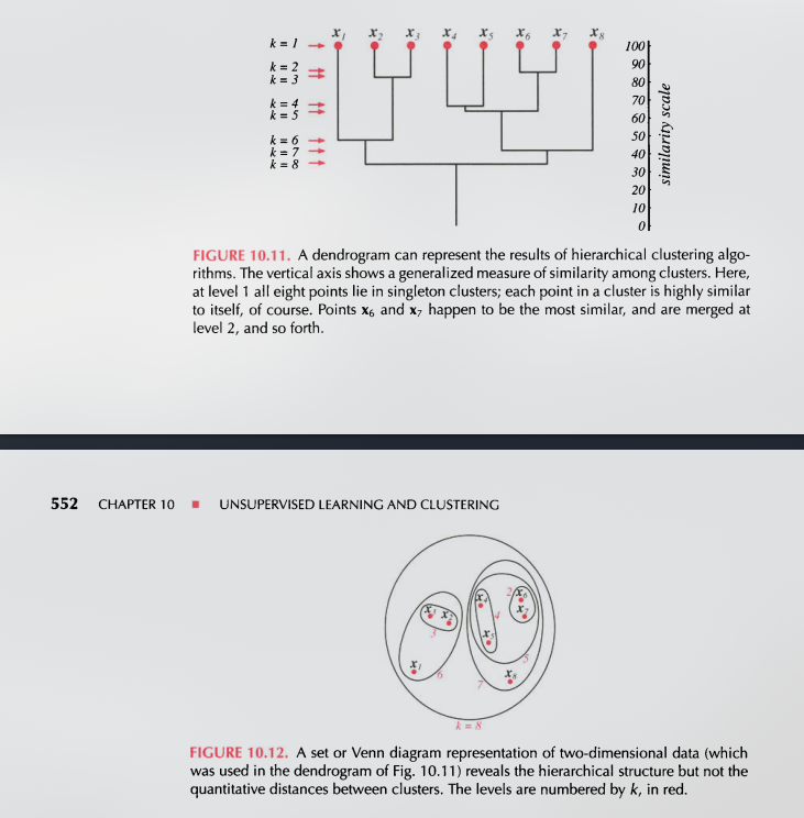
Image taken from Pattern Classification

The vertical axis of the dendrogram represents the cluster distance or dissimilarity. This is the value of the linkage criterion at which each merge occurred. By drawing a horizontal line across the dendrogram, one can "cut" the tree to obtain a specific number of clusters. A cut at a lower distance threshold results in a larger number of smaller clusters, reflecting a finer granularity. A cut at a higher distance results in fewer, larger clusters.

Measuring Distance Between Clusters (Linkage Criteria)

• Single Linkage: This method can identify clusters of non-elliptical shapes but is sensitive to noise and can result in long, drawn-out clusters, a phenomenon known as the "chaining effect".

  $$D(c_1,c_2)=\underset{x_1\in c_1,x_2\in c_2}{min}D(x_1,x_2)$$

• Complete Linkage: This approach is less susceptible to the chaining effect and tends to produce more compact, roughly spherical clusters.

  $$D(c_1,c_2)=\underset{x_1\in c_1,x_2\in c_2}{max}D(x_1,x_2)$$

• Average Linkage: The distance is calculated as the average of all pairwise distances between the points in the two clusters. This serves as a compromise between the single and complete linkage methods and is generally less sensitive to outliers.

  $$D(c_1,c_2)=\frac{1}{|c_1||c_2|}\sum _{x_1\in c_1}\sum _{x_2\in c_2}D(x_1,x_2)$$

• Ward's Method: This method takes a different approach based on variance. It merges the pair of clusters that leads to the minimum increase in the total within-cluster variance. The variance is measured as the sum of squared differences between the points and the centroid of a cluster. The increase in the sum of squared errors (SSE) when merging two clusters, $c_a$ and $c_b$, is:

  $$\mathrm{\Delta }(c_a,c_b)=\sum _{x\in c_a\cup c_b}\parallel x-{\mu }_{ab}{\parallel }^2-\sum _{x\in c_a}\parallel x-{\mu }_a{\parallel }^2-\sum _{x\in c_b}\parallel x-{\mu }_b{\parallel }^2$$

  where $\mu$ is the centroid of a cluster. This can be simplified to:

  $$\mathrm{\Delta }(c_a,c_b)=\frac{|c_a||c_b|}{|c_a|+|c_b|}\parallel {\mu }_a-{\mu }_b{\parallel }^2$$

  Ward's method tends to produce clusters that are compact and of similar size.

"AI AI CAPTAIN!"