Optimal Demodulation & Performance

this is first coz i forget lol

Signal Space and AWGN Model

• Core Idea: Represent $M$ possible transmitted continuous-time signals $s_i(t)$ as vectors ${\mathbf{s}}_i$ in an $n$-dimensional signal space ($n\le M$).
• AWGN Channel Model (Vector Form): The received vector $\mathbf{Y}$ when signal ${\mathbf{s}}_i$ is sent is:$$\mathbf{Y}={\mathbf{s}}_i+\mathbf{N}$$
  • $\mathbf{N}$ is the noise vector. Its components $N[k]$ are i.i.d. Gaussian $N(0,{\sigma }^2)$.
  • The noise variance per real dimension is related to the physical noise PSD $N_0$ by ${\sigma }^2=N_0/2$.

Optimal Decision Rules (Minimizing Probability of Error)

• MAP (Maximum A Posteriori) Rule: Optimal overall. Requires prior probabilities ${\pi }_i=P(H_i)$. Choose hypothesis $i$ that maximizes the posterior probability $P(H_i|\mathbf{y})$.
  • Decision Metric (Equivalent): Choose $i$ that maximizes:$${\mathrm{\Lambda }}_{MAP}(i)=⟨\mathbf{y},{\mathbf{s}}_i⟩-\frac{1}{2}\parallel {\mathbf{s}}_i{\parallel }^2+{\sigma }^2\ln ({\pi }_i)$$
  • Vector Form: Choose $i$ that minimizes:$$d_{MAP}^2(i)=\parallel \mathbf{y}-{\mathbf{s}}_i{\parallel }^2-2{\sigma }^2\ln ({\pi }_i)$$
• ML (Maximum Likelihood) Rule: Optimal when priors ${\pi }_i=1/M$ are equal. Chooses hypothesis $i$ that maximizes the likelihood $p(\mathbf{y}|H_i)$.
  • Decision Metric (Equivalent): Choose $i$ that maximizes:$${\mathrm{\Lambda }}_{ML}(i)=⟨\mathbf{y},{\mathbf{s}}_i⟩-\frac{1}{2}\parallel {\mathbf{s}}_i{\parallel }^2$$
  • Vector Form (Minimum Distance Rule): Choose $i$ that minimizes:$$d_{ML}^2(i)=\parallel \mathbf{y}-{\mathbf{s}}_i{\parallel }^2$$
• Implementation: Using a bank of correlators (computing $⟨y,s_i⟩$) or matched filters (output sampled at peak = $⟨y,s_i⟩$).

Performance Metrics: Geometry and SNR

Euclidean Distance

• The distance between signal points in the constellation is crucial for performance.$$d_{ij}=\parallel {\mathbf{s}}_i-{\mathbf{s}}_j\parallel$$
• Minimum Distance ($d_{min}$): The smallest distance between any two distinct constellation points. Often dominates performance at high SNR.$$d_{min}=\underset{i\ne j}{min}\{d_{ij}\}$$

Energy per Bit ($E_b$)

• Relates average signal energy to the information transmitted.
• Average Energy per Symbol: $E_s=\frac{1}{M}\sum _{i=0}^{M-1}\parallel {\mathbf{s}}_i{\parallel }^2$ (assuming equal priors).
• Energy per Bit:$$E_b=\frac{E_s}{{\log }_{2}M}$$
  • $E_b$ represents the energy required per information bit.

Noise Power Spectral Density ($N_0$)

• Fundamental measure of noise level (power per Hz, one-sided). Directly related to noise variance per dimension: ${\sigma }^2=N_0/2$.

Q-Function

• Tail probability of a standard Normal distribution $N(0,1)$. Used to express error probabilities involving Gaussian noise.$$Q(x)={\int }_x^{\mathrm{\infty }}\frac{1}{\sqrt{2\pi }}{e}^{-u^2/2}du=\frac{1}{2}\text{erfc}\left(\frac{x}{\sqrt{2}}\right)$$

Performance Formulas (ML, Equal Priors)

Pairwise Error Probability (PEP)

• The probability of deciding ${\mathbf{s}}_j$ when ${\mathbf{s}}_i$ was sent, assuming only these two possibilities exist.$$P({\mathbf{s}}_i\to {\mathbf{s}}_j)=Q\left(\frac{d_{ij}}{2\sigma }\right)=Q\left(\frac{d_{ij}}{\sqrt{2N_0}}\right)$$

Binary Signaling Error Probability ($M=2$)

• Directly uses the pairwise error probability with $d=d_{01}$.$$P_e=Q\left(\frac{d}{\sqrt{2N_0}}\right)$$

M-ary Symbol Error Rate (SER, $P_e$) - Approximations

• Exact calculation is complex. Bounds and approximations are used.
• Union Bound: Upper bounds the probability of error by summing PEPs.$$P_{e|i}\le \sum _{j\ne i}Q\left(\frac{d_{ij}}{\sqrt{2N_0}}\right)$$
  • Average SER: $P_e=\sum _i{\pi }_i{P}_{e|i}\le \sum _i{\pi }_i\sum _{j\ne i}Q\left(\frac{d_{ij}}{\sqrt{2N_0}}\right)$
• Nearest Neighbor Approximation (High SNR): Assumes errors are dominated by mistaking a signal for one of its nearest neighbors at distance $d_{min}$.$$P_e\approx {\overline{N}}_{min}Q\left(\frac{d_{min}}{\sqrt{2N_0}}\right)$$
  • ${\overline{N}}_{min}$: Average number of nearest neighbors at distance $d_{min}$.

Efficiency Metrics

Power Efficiency (${\eta }_P$)

• Concept: How effectively does the constellation use energy to create distance between points? A measure of noise immunity for a given $E_b$. Often implicitly compares to BPSK.
• Formal Definition (Binary Context): For binary signaling, we related $P_e$ to ${\eta }_P$:$$P_e=Q\left(\sqrt{\frac{2{\eta }_P{E}_b}{N_0}}\right)\text{where }{\eta }_P=\frac{d^2}{4E_b}$$
  • For antipodal BPSK, ${\eta }_P=1$. For orthogonal/OOK, ${\eta }_P=1/2$.
• M-ary Context: Instead of defining a single ${\eta }_P$, performance is typically analyzed via $d_{min}$ and $E_b$. The quantity $\frac{d_{min}^2}{E_b}$ acts as a figure of merit for power efficiency when comparing constellations (higher is better). It tells us how much squared minimum distance we get per unit of energy-per-bit.
  • From the NN approx: $P_e\approx {\overline{N}}_{min}Q(\sqrt{\frac{d_{min}^2/E_b}{2N_0/E_b}}\times \frac{E_b}{N_0})\approx {\overline{N}}_{min}Q\left(\sqrt{\frac{d_{min}^2}{E_b}\frac{E_b}{2N_0}}\right)$.
  • For high SNR, the argument of the Q-function dominates. Larger $d_{min}^2/E_b$ leads to smaller $P_e$ for the same $E_b/N_0$.

Bandwidth Efficiency (${\eta }_B$)

• Concept: How many bits are sent per second per Hertz of bandwidth?
• Formula (using Nyquist minimum bandwidth $B_{min}=R_s/2=1/(2T)$ for complex signals):$${\eta }_B=\frac{R_b}{B_{min}}=\frac{({\log }_{2}M)/T}{1/(2T)}=2{\log }_{2}M(\text{bits/sec/Hz, complex/2D)}$$
  • For real baseband (1D): ${\eta }_B={\log }_{2}M$.
  • If excess bandwidth $\alpha$ is used: $B=(1+\alpha )B_{min}$, so ${\eta }_B=\frac{2{\log }_{2}M}{1+\alpha }$ (complex).

Linkages and Tradeoffs

• Pe vs. Geometry & SNR: The error probability $P_e$ fundamentally depends on the ratio of minimum distance ($d_{min}$) to noise standard deviation ($\sigma =\sqrt{N_0/2}$).$$P_e\approx {\overline{N}}_{min}Q\left(\frac{d_{min}}{\sqrt{2N_0}}\right)$$
• Pe vs. $E_b/N_0$: We typically express performance as $P_e$ vs. $E_b/N_0$. The relationship involves the constellation geometry via $d_{min}^2/E_b$:$$\frac{d_{min}}{\sqrt{2N_0}}=\sqrt{\frac{d_{min}^2}{2N_0}}=\sqrt{\frac{d_{min}^2}{E_b}\frac{E_b}{2N_0}}$$
  • A constellation with a higher $d_{min}^2/E_b$ (better power efficiency) will achieve a lower $P_e$ for the same $E_b/N_0$.
• Power-Bandwidth Tradeoff:
  • Increasing constellation size $M$ generally increases bandwidth efficiency (${\eta }_B$).
  • Increasing constellation size $M$ (for PAM, PSK, QAM) generally decreases power efficiency (reduces $d_{min}^2/E_b$) because points are packed closer for the same average energy $E_s$.
  • Orthogonal signaling is an exception (power efficiency improves with M, bandwidth efficiency decreases).

Analog Modulation

Things to Remember

• Don't just blindly apply Carson, there could be cases where the signal isn't symmetric, remember the formula isn't 2(B+fmax) but 2(B+fmax+ - fmin-).

Chapter 1: Introduction

Basic Communication System

• Goal: Transfer information reliably and efficiently from a Source to a Destination across a Channel.
• Fundamental Blocks: Source $\to$ Transmitter $\to$ Channel $\to$ Receiver $\to$ Destination.
• Transmitter: Encodes source information into a signal suitable for the channel (modulation).
• Channel: The physical medium (wire, fiber, air, storage medium, etc.) that carries the signal. Introduces challenges.
• Receiver: Processes the received (corrupted) signal to estimate the original information (demodulation, decoding).
• Information Transfer: Can be across space (telephony, broadcasting, internet browsing) or time (data storage like CDs, DVDs, hard drives, cloud).

The Channel: Resource and Challenge

• The channel is the resource enabling communication but presents challenges.

Channel Challenge: Limited Spectrum/Bandwidth

• Physical media cannot support infinite frequencies. Transmission must occur within allocated/supported bands.
• Wired: Medium characteristics impose inherent frequency limits (e.g., high-frequency attenuation in copper pairs).
• Wireless: A scarce, regulated resource. Different frequency bands have different properties:
  • Low frequencies: Require large antennas, offer low bandwidth.
  • High frequencies: Suffer high attenuation, require line-of-sight (esp. > 5 GHz).
• Motivation: Leads to the need for bandwidth-efficient communication techniques and spectrum sharing strategies.

Channel Challenge: Noise and Interference

• Noise: Unavoidable random perturbations corrupting the signal.
  • Thermal Noise: Fundamental, due to random motion of electrons.
  • Other Sources: Man-made EMI, powerline interference, cosmic noise, shot noise.
  • Model: Typically modelled as Additive White Gaussian Noise (AWGN). Additive ($y(t)=x(t)+\eta (t)$), White (flat Power Spectral Density, PSD), Gaussian (amplitude distribution).
• Interference: Signals from other users/systems sharing the medium.
• Motivation: Need for techniques robust to noise and interference (e.g., signal design, error control coding, spread spectrum).

Channel Challenge: Distortion

• Attenuation: Signal weakening with distance/frequency. Varies across different frequencies in wired/wireless channels.
• Multipath (Wireless): Signal arrives via multiple paths due to reflections. Causes:
  • Time-varying channel gain (fading).
  • Delay spread: Symbols interfere with subsequent symbols (Inter-Symbol Interference - ISI).
• Linear Time-Invariant (LTI) Model: Often used for wired channels or short-duration wireless channels. $y(t)=h(t)\ast x(t)+\eta (t)$.
• Linear Time-Variant (LTV) Model: Needed for wireless channels with mobility. $y(t)=h(\tau ;t)\ast x(t)+\eta (t)$.
• Motivation: Requires equalization techniques at the receiver to combat distortion and ISI.

Channel Challenge: Sharing and Limited Capacity

• Sharing: Wireless/wired resources often need to be shared among many users (e.g., cellular, WiFi, Ethernet). Leads to congestion, collisions, need for multiple access protocols.
• Limited Capacity (Shannon's Theorem): Defines the maximum theoretical rate (bits/sec) for reliable communication over a noisy channel.$$C=B{\log }_2(1+\text{SNR})$$
  • Fundamental trade-off between bandwidth ($B$), signal power ($P$ or $S$), noise power ($N$), and data rate ($C$).
• Motivation: Benchmarks performance, drives search for efficient coding/modulation, highlights resource limitations.

Analog vs. Digital Communication

• Analog: Information (message signal) is a continuous-time, continuous-valued waveform (e.g., speech, audio). Transmitter directly maps message to transmitted analog signal.
  • Examples: AM/FM radio, analog TV, vinyl records, 1st gen cellular (AMPS).
  • Simple: Conceptually straightforward (Fig 1.1 / Slide 38).
  • Susceptible to Noise: Noise accumulates through repeaters.
• Digital: Information (message signal) is represented by discrete values (often bits). Analog signals are first converted (sampled & quantized).
  • Examples: Modern cellular (2G onwards), digital TV/radio, CDs/DVDs, data networks.
  • Digital System Blocks (Fig 1.2 / Slide 41): Source Encoder (Compression) $\to$ Channel Encoder (Error Control) $\to$ Modulator $\to$ Channel $\to$ Demodulator $\to$ Channel Decoder $\to$ Source Decoder.
  • Source Encoder: Converts source info to bits efficiently (removes redundancy). E.g., Huffman coding, ZIP, JPEG, MP3.
  • Channel Encoder: Adds controlled redundancy tailored to the channel for error detection/correction. E.g., repetition code.
  • Modulator: Maps bits/symbols to analog waveforms suitable for the channel (deals with bandwidth/power constraints).
  • Demodulator/Decoder: Reverse processes at the receiver.
• Why Digital? (Sec 1.1.3 / Slide 53):
  • Robustness: Regenerative repeaters clean noise/distortion perfectly (if errors are corrected).
  • Optimality (Source-Channel Separation): Design source coding (compression) and channel coding (error control + modulation) independently for optimal performance (huge gains). Not possible in analog.
  • Scalability & Flexibility: Networking (Internet relies on digital packets), integration of diverse services, easy storage, DSP implementation, cheaper hardware.
  • Performance: Arbitrarily low error rates possible via channel coding (Shannon's theorem).
  • Security: Encryption is readily applied to digital data.
• Role for Analog: Physical world and channels are analog. Digital systems need analog front-ends: DACs, ADCs, amplifiers, mixers, filters, antennas. RF/analog design remains crucial (Sec 1.1.4).

Chapter 2: Signals and Systems Fundamentals

Signal Representations (Sec 2.2)

• Continuous Time (CT): $x(t)$
• Discrete Time (DT): $x[n]$ (often from sampling $x(n{T}_s)$)
• Indicator Function: $I_A(x)=1$ if $x\in A$, $0$ otherwise. Used for defining pulses, e.g., $I_{[0,T]}(t)$. (Slide 73)
• Sinusoid: Basic periodic signal $s(t)=A\cos (2\pi f_{c}t+\theta )$.
  • Polar Form: Amplitude $A$, frequency $f_c$, phase $\theta$.
  • Rectangular Form: $s(t)=A_c\cos (2\pi f_{c}t)-A_s\sin (2\pi f_{c}t)$.
  • Complex Representation: $A{e}^{j\theta }=A_c+j{A}_s$. (Slide 75)
• Complex Exponential: $s(t)=\alpha e^{j2\pi f_{c}t}$ where $\alpha =A{e}^{j\theta }$. Contains amplitude and phase. $s(t)=\text{Re}\{s(t)\}$ gives the real sinusoid. (Slide 76)
• Delta Function $\delta (t)$: Idealized impulse. Defined by sifting property $\int s(t)\delta (t-t_0)dt=s(t_0)$.
• Sinc Function: $\text{sinc}(x)=\frac{\sin (\pi x)}{\pi x}$. (Note: definition varies; this is common in comms).

Inner Product, Energy, Power (Sec 2.2)

• Inner Product (CT): $⟨s,r⟩={\int }_{-\mathrm{\infty }}^{\mathrm{\infty }}s(t)r^{\ast }(t)dt$. (Slide 77)
• Energy (CT): $E_s=\parallel s{\parallel }^2=⟨s,s⟩={\int }_{-\mathrm{\infty }}^{\mathrm{\infty }}|s(t){|}^{2}dt$. (Slide 78)
• Power (CT, for signals not having finite energy): Time average of energy.$$P_s=\underset{T_0\to \mathrm{\infty }}{lim}\frac{1}{T_0}{\int }_{-T_0/2}^{T_0/2}|s(t){|}^{2}dt=\overline{|s(t){|}^2}\$\$(Slide80,81)$$
• DC Value: $\overline{s(t)}$. Zero for sinusoids with $f_c\ne 0$.

LTI Systems and Convolution (Sec 2.3)

• Linear Time-Invariant (LTI): Output is convolution of input $x(t)$ and impulse response $h(t)$.$$y(t)=x(t)\ast h(t)={\int }_{-\mathrm{\infty }}^{\mathrm{\infty }}x(\tau )h(t-\tau )d\tau$$
• Frequency Domain: $Y(f)=X(f)H(f)$. (Slide 89)
• Complex Exponentials are Eigenfunctions: $e^{j2\pi f_{0}t}\ast h(t)=H(f_0)e^{j2\pi f_{0}t}$.

Fourier Analysis (Sec 2.4, 2.5)

• Fourier Series (Periodic Signals): $u(t)=\sum _{n=-\mathrm{\infty }}^{\mathrm{\infty }}{u}_n{e}^{j2\pi n{f}_{0}t}$. (Slide 84)
• Fourier Transform (Aperiodic/Finite Energy): (Slide 85)$$U(f)={\int }_{-\mathrm{\infty }}^{\mathrm{\infty }}u(t)e^{-j2\pi ft}dt\leftrightarrow u(t)={\int }_{-\mathrm{\infty }}^{\mathrm{\infty }}U(f)e^{j2\pi ft}df$$
• Properties: Linearity, Time/Freq Shift, Differentiation, Parseval, Convolution <=> Multiplication. (Slides 86-89)
• Key Pairs: $\delta (t)\leftrightarrow 1$; $e^{j2\pi f_{0}t}\leftrightarrow \delta (f-f_0)$; $I_{[-T/2,T/2]}(t)\leftrightarrow T\text{sinc}(fT)$. (Slide 91)

Spectral Density and Bandwidth (Sec 2.6)

• ESD (Finite Energy): ${\mathcal{E}}_u(f)=|U(f){|}^2$. Total Energy $E_u=\int {\mathcal{E}}_u(f)df$. (Slide 102)
• PSD (Finite Power / WSS Processes): $S_X(f)=\mathcal{F}\{R_X(\tau )\}$. Total Power $P_X=\int S_X(f)df$.
• Bandwidth: Defines frequency occupancy.
  • Strictly Bandlimited: $U(f)=0$ outside a band. (Slide 104, 105)
  • Fractional Power Containment: Smallest band containing $X\mathrm{\%}$ of energy/power. (Slide 107)
  • 3dB Bandwidth: Width where $|U(f){|}^2$ is above half its peak value. (Slide 108)
  • For Real Signals: Only positive frequencies count (one-sided bandwidth). (Slide 105)
  • For Complex Signals: Both positive and negative frequencies count. (Slide 106)

Baseband and Passband (Sec 2.7)

• Baseband Signal: Spectrum concentrated around DC. $U(f)\approx 0$ for $|f|>W$. (Slide 110)
  • Examples: Source signals (speech, audio), baseband digital pulses. (Slide 111)
• Passband Signal: Spectrum concentrated around $\pm f_c$, away from DC. $U(f)\approx 0$ for $|f\pm f_c|>W$, with $f_c>W$. (Slide 112)
  • Examples: Modulated signals for wireless transmission. (Slide 113, 114)
• Channels: Can also be baseband (e.g., twisted pair) or passband (e.g., wireless channel allocation). (Slide 116, 117)

Complex Baseband Representation (Sec 2.8)

• Motivation: Unify analysis of baseband and passband signals/systems. Most signal processing happens in complex baseband. (Slide 118)
• Representation: Real passband $u_p(t)$ $\leftrightarrow$ Complex baseband $u(t)$.$$u_p(t)=\text{Re}\{u(t)e^{j2\pi f_{c}t}\}$$
• Three Views (Slide 130, 131):
  1. I/Q Components (Rectangular): $u(t)=u_c(t)+j{u}_s(t)$.
     $u_p(t)=u_c(t)\cos (2\pi f_{c}t)-u_s(t)\sin (2\pi f_{c}t)$. (Slide 123)
  2. Envelope and Phase (Polar): $u_c(t)=e(t)\cos \theta (t)$, $u_s(t)=e(t)\sin \theta (t)$.
     $u_p(t)=e(t)\cos (2\pi f_{c}t+\theta (t))$. (Slide 128)
  3. Complex Envelope: $u(t)=e(t)e^{j\theta (t)}$. Links the two. (Slide 129)
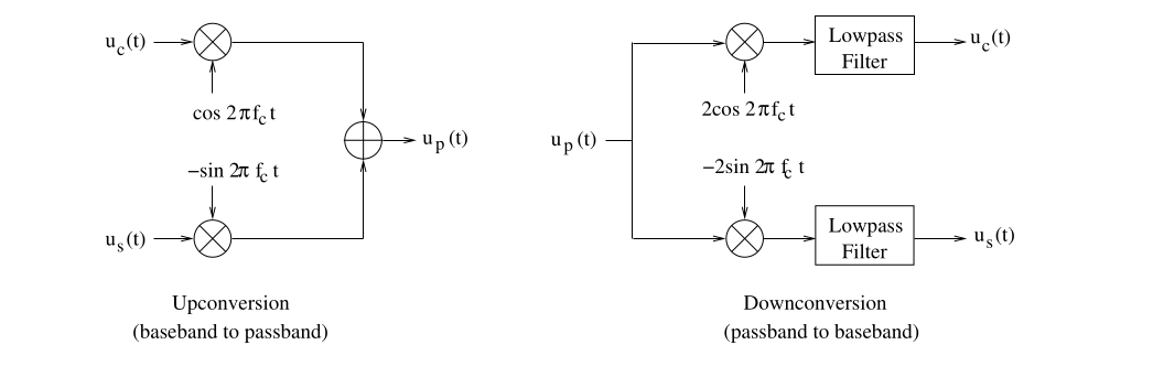
• Orthogonality: $\cos (2\pi f_{c}t)$ and $\sin (2\pi f_{c}t)$ carriers are orthogonal. Allows independent transmission on I and Q. (Slide 125)
• Upconversion/Downconversion (Modulation/Demodulation): (Slide 126, 127)
  • Multiply by $\cos$ and $\sin$ carriers, then use LPFs.
• Effect of Frequency/Phase Offset: If local oscillator has offset $\mathrm{\Delta }f$ and phase offset $\gamma$, i.e., $\varphi (t)=2\pi \mathrm{\Delta }ft+\gamma$, the received complex envelope is rotated: $\tilde{u}(t)=u(t)e^{j\varphi (t)}$. This mixes I/Q components. (Slide 132)
  • Requires Coherent Detection: Receiver must synchronize its LO frequency and phase ($\mathrm{\Delta }f\approx 0,\gamma \approx 0$) or compensate for the offset. (Slide 133)
• Frequency Domain: (Slide 135, 136, 137)$$U_p(f)=\frac{1}{2}[U(f-f_c)+U^{\ast }(-f-f_c)]$$
  • Reconstruction: $U(f)=2U_p^{+}(f+f_c)$ where $U_p^{+}$ is positive frequency part.
• Filtering Equivalence: Passband filtering $y_p(t)=u_p(t)\ast h_p(t)$ is equivalent (up to scaling) to complex baseband filtering $y(t)=\frac{1}{2}u(t)\ast h(t)$. Implemented using 4 real convolutions. (Slide 139, 141)
• Energy/Power: $E_{u_p}=\frac{1}{2}{E}_u$. (Slide 142)
• Correlation: $⟨u_p,v_p⟩=\frac{1}{2}\text{Re}\{⟨u,v⟩\}$. (Slide 143)
• Modern Architecture: DSP operates on complex baseband samples. (Slide 144)

Chapter 3: Analog Communication Techniques

Motivation (Slide 148)

• Understand underlying physical signals even in digital era.
• Common language with circuit designers.
• Analog-centric techniques critical when pushing limits (low power, high speed).
• Concepts like PLL, Superhet remain relevant.

Terminology (Sec 3.1 / Slides 149-151)

• Message Signal: $m(t)$, real-valued, baseband, often assumed zero mean ($\overline{m}=0$). Power $P_m=\overline{m^2(t)}$.
• Transmitted Signal: $u_p(t)$, passband. Can be written via I/Q ($u_c,u_s$) or Env/Phase ($e(t),\theta (t)$).

Amplitude Modulation (AM) (Sec 3.2)

DSB-SC (Double Sideband Suppressed Carrier) (Sec 3.2.1)

• Generation: $u_{DSB}(t)=Am(t)\cos (2\pi f_{c}t)$. Complex envelope $u(t)=Am(t)$. (Slide 156)
• Spectrum: $U_{DSB}(f)=\frac{A}{2}[M(f-f_c)+M(f+f_c)]$. $BW=2B$. (Slide 157, 159)
• Demodulation: Requires coherent detector. Multiply by $2\cos (2\pi f_{c}t+{\theta }_r)$, then LPF. Output $m_{out}(t)\propto m(t)\cos {\theta }_r$. Needs phase sync. (Slide 160, 164)

Conventional AM (Sec 3.2.2)

• Generation: $u_{AM}(t)=A_c(1+a{m}_n(t))\cos (2\pi f_{c}t)$. Large carrier added. (Slide 166)
• Spectrum: DSB spectrum + impulses at $\pm f_c$. (Slide 167)
• Envelope Detection: If modulation index $a\le 1$, envelope $e(t)=A_c(1+a{m}_n(t))$. Recover message with simple diode+RC circuit. (Slide 168-171, 173, 175, 176, 180, 181)
• Modulation Index: $a=\frac{A|m(t{)}_{min}|}{A_c}\le 1$. (Slide 173)
• RC Time Constant: $\frac{1}{f_c}\ll RC\ll \frac{1}{B}$. (Slide 177, 181)
• Power Efficiency: Low due to carrier power. ${\eta }_{AM}=\frac{a^2\overline{m_n^2}}{1+a^2\overline{m_n^2}}$. (Slide 192)
• Modulators: Can use non-linear devices or switching modulators instead of ideal multipliers. (Slide 185-188)

SSB (Single Sideband) (Sec 3.2.3)

• Motivation: $BW=B$. Most bandwidth efficient AM. (Slide 199)
• Generation:
  • Filtering: Ideal filter removes one sideband (hard). (Slide 200, 201)
  • Phase Shift: $u_{USB/LSB}(t)=m(t)\cos (2\pi f_{c}t)\mp \hat{m}(t)\sin (2\pi f_{c}t)$. Uses Hilbert Transform. (Slide 208-211, 216, 217)
• Complex Envelope: $u_{USB/LSB}(t)=m(t)\pm j\hat{m}(t)$. (Slide 217)
• Demodulation: Coherent detection needed. Very sensitive to phase errors (crosstalk + attenuation). (Slide 221) Envelope detection possible if large carrier added. (Slide 222)

QAM (Quadrature Amplitude Modulation) (Sec 3.2.5)

• Generation: $u_{QAM}(t)=m_c(t)\cos (2\pi f_{c}t)-m_s(t)\sin (2\pi f_{c}t)$. Two independent messages. (Slide 224)
• Complex Envelope: $u(t)=m_c(t)+j{m}_s(t)$.
• Demodulation: Coherent detection needed. Sensitive to phase errors (crosstalk). (Slide 226)

VSB (Vestigial Sideband) (Sec 3.2.4)

• Compromise between SSB (bandwidth) and DSB (filter simplicity). (Slide 228)
• Filter leaves a "vestige" of the unwanted sideband.
• Design criterion: $H_p(f-f_c)+H_p(f+f_c)=\text{constant}$ over message band ensures $m(t)$ recovered as I component. (Slide 229)

Angle Modulation (Sec 3.3)

• Constant envelope $u_p(t)=A_c\cos (2\pi f_{c}t+\theta (t))$. Information in phase $\theta (t)$. (Slide 235, 237)
• Phase Modulation (PM): $\theta (t)=k_{p}m(t)$.
• Frequency Modulation (FM): Instantaneous frequency $f_i(t)=f_c+f(t)=f_c+k_{f}m(t)$. $\theta (t)=2\pi k_f\int m(\tau )d\tau$.
• Equivalence: FM is PM with integrated message; PM is FM with differentiated message. (Slide 238-240)
• Non-linearity: Angle modulation is a non-linear operation. (Slide 242)
• Preference: FM preferred for analog (smoother phase); PM often base for digital (PSK). (Slide 243, 244)
• Modulation Index (FM): $\beta =\mathrm{\Delta }{f}_{max}/B$. (Slide 246)
• Bandwidth:
  • Narrowband FM ($\beta \ll 1$): $BW\approx 2B$. Similar to AM.
  • Wideband FM ($\beta \gg 1$): $BW\approx 2\mathrm{\Delta }{f}_{max}$. Dominated by frequency deviation.
  • Carson's Rule: General estimate $B{W}_{FM}\approx 2(\mathrm{\Delta }{f}_{max}+B)=2B(\beta +1)$. (Slide 260, 263)
• Spectrum (Sinusoidal Message): Involves Bessel functions $J_n(\beta )$. Complex envelope spectrum $U(f)=\sum J_n(\beta )\delta (f-n{f}_m)$. (Slide 264-268)
• Modulation: Typically uses VCO (Voltage Controlled Oscillator). Direct or Indirect FM. (Slide 247)
• Demodulation:
  • Limiter-Discriminator: Limiter removes amplitude variation, Discriminator converts freq variations to amplitude variations (e.g., differentiator + envelope detector, or slope detector). (Slide 250-252)
  • PLL (Phase Locked Loop).

Receiver Architectures (Sec 3.4)

• Superheterodyne: Mix RF to fixed IF. Principle: Sloppy RF filter (image reject), sharp IF filter (channel select). Tradeoff between image rejection and adjacent channel rejection based on IF choice. (Slide 279, 284, 287, 289)
• Mixer: Non-linear device creating sum and difference frequencies. (Slide 285)
• Image Frequency: $f_{IM}=f_{RF}\pm 2f_{IF}$. Unwanted signal that also mixes down to IF. Must be rejected by RF filter.
• Direct Conversion: Mix directly to baseband (zero-IF). Avoids image issue, simpler integration. Challenges: DC offset, LO leakage, 1/f noise. (Slide 291, 292)
• mmWave: May revive Superhet due to ADC limitations, or use hybrid architectures. (Slide 293)

Phase Locked Loop (PLL) (Sec 3.5)

• Concept: Feedback loop: Phase Detector compares input phase ${\theta }_i$ and VCO output phase ${\theta }_o$; error drives VCO via Loop Filter. (Slide 296, 297)
• Phase Detectors: Mixer-based (output $\propto \sin ({\theta }_i-{\theta }_o)$) or logic-based (XOR, phase-frequency detector). (Slide 298-302)
• Applications: (Slide 125)
  • FM Demodulation: VCO input tracks message $m(t)$ if loop tracks ${\theta }_i(t)=2\pi k_f\int m$. (Slide 304)
  • Frequency Synthesis: Use frequency divider in loop to synthesize high frequency LO from stable low frequency reference. (Slide 305)
• Mathematical Model: Non-linear due to phase detector. (Slide 308)
• Linearized Model: Assumes small phase error $\sin ({\theta }_e)\approx {\theta }_e$. Allows LTI analysis using Laplace transforms. (Slide 309-312)
• Loop Order & Tracking:
  • 1st Order (G(s)=1): Tracks phase steps with zero steady-state error. Cannot track frequency steps (has steady-state phase error $2\pi \mathrm{\Delta }f/K$). (Slide 313, 314, 315)
  • 2nd Order (G(s)=1+a/s): Tracks frequency steps with zero steady-state phase error. (Slide 316, 317)
• Non-linear Behavior: Locking range depends on loop gain K vs frequency offset $\mathrm{\Delta }f$. Phase plane analysis useful. (Slide 321-324)

Chapter 4: Digital Modulation

Signal Constellations (Sec 4.1)

• Mapping bits to complex symbols $b[n]=b_c[n]+j{b}_s[n]$. Plotted on I/Q plane. (Slide 331, 338)
• Linear Baseband Model: $u(t)=\sum b[n]p(t-nT)$. (Slide 328)
• Linear Passband Model: $u_p(t)=\text{Re}\{u(t)e^{j2\pi f_{c}t}\}$. (Slide 329)
• Examples:
  • BPSK (2-PAM): $b[n]\in \{\pm 1\}$. Baseband or Passband (phase shifts 0, $\pi$). (Slide 330, 332)
  • 4-PAM: $b[n]\in \{\pm 1,\pm 3\}$. Baseband. (Slide 333)
  • QPSK (4-PSK / 4-QAM): $b[n]\in \{\pm 1\pm j\}$. Passband (phase shifts $\pm \pi /4,\pm 3\pi /4$). (Slide 334, 335, 336, 337)
  • M-PSK: Points on a circle.
  • M-QAM: Points on a grid.

Bandwidth Occupancy (Sec 4.2)

• Requires statistical description (symbols $b[n]$ are random).
• Power Spectral Density (PSD): Characterizes power distribution vs frequency for finite power signals / WSS processes. (Slide 342)
• Periodogram Estimation: Estimate PSD from finite observation window $T_0$: ${\hat{S}}_x(f)=|X_{T_0}(f){|}^2/T_0$. PSD is limit as $T_0\to \mathrm{\infty }$. (Slide 343)
• PSD of Linearly Modulated Signal (Thm 4.2.1): If symbols are zero mean and uncorrelated with average energy ${\sigma }_b^2$:$$S_u(f)=\frac{{\sigma }_b^2}{T}|P(f){|}^2$$
  • Power $P_u=\frac{{\sigma }_b^2}{T}\parallel p{\parallel }^2$. (Slide 344)
• Bandwidth Definitions based on PSD: (Slide 347)
  • 3dB Bandwidth.
  • Fractional Power Containment Bandwidth.
• Time/Frequency Normalization: Analyze system with $T=1$, then scale bandwidth by $1/T$. (Slide 348, 349)
• Example: Rectangular Pulse: $p_1(t)=I_{[0,1]}(t)⟹S_{u1}(f)={\sigma }_b^2{\text{sinc}}^2(f)$. Wide tails, poor bandwidth containment. (Slide 350)
• Example: Sine Pulse: $p_1(t)=\sqrt{2}\sin (\pi t)I_{[0,1]}(t)⟹S_{u1}(f)$ has much better decay. (Slide 353)

Design for Bandlimited Channels (Sec 4.3)

• Motivation: Match signal spectrum to channel bandwidth, avoid ISI. (Slide 371, 372)
• Nyquist Sampling Theorem (Thm 4.3.1): Signal bandlimited to $W/2$ is determined by samples at rate $W$. $s(t)=\sum s(n/W)\text{sinc}(W(t-n/W))$. (Slide 368)
  • Implies $W$ complex dimensions / second in bandwidth $W$.
• Nyquist Criterion for Zero ISI (Thm 4.3.2): (Slide 376)
  • Time: $p(kT)=\delta [k]$ (pulse zero crossings).
  • Frequency: $\frac{1}{T}\sum _{k}P(f-k/T)=1$. (Aliased spectrum is flat).
• Sinc Pulse: $p(t)=\text{sinc}(t/T)$. Minimum BW $1/(2T)$. Problem: Slow decay causes large ISI with timing errors. (Slide 369, 375, 381, 382)
• Need for Excess Bandwidth: Pulses decaying faster than $1/t$ (like $1/t^2$ or $1/t^3$) require bandwidth $>1/(2T)$ but mitigate ISI issues. (Slide 385)
• Trapezoidal Pulse (Freq): Convolution of two rects. $p(t)=\text{sinc}(at/T)\text{sinc}(bt/T)$. Decays as $1/t^2$. (Slide 386-389)
• Raised Cosine (RC) Pulse (Freq): Smoother rolloff than trapezoid. $p(t)=\text{sinc}(t/T)\frac{\cos (\pi \alpha t/T)}{1-(2\alpha t/T{)}^2}$. Decays as $1/t^3$. (Slide 395, 396)
• Excess Bandwidth ($\alpha$): Factor by which BW exceeds minimum $1/(2T)$. $BW=\frac{1+\alpha }{2T}$.
• Nyquist Rate Property: A pulse Nyquist at rate $1/T$ is also Nyquist at rates $1/(KT)$ for integer $K>1$. (Slide 390)

Bandwidth Efficiency (Sec 4.3.3)

• ${\eta }_B=\frac{\text{bits/symbol}}{\text{dimensions/symbol}}=\frac{{\log }_{2}M}{N_D}$. For complex baseband, $N_D=1$ complex dim, or 2 real dims.
• For Nyquist pulse with excess $\alpha$, using $N_D=BW/(1/(2T))=1+\alpha$ dimensions/symbol seems intuitive but the standard definition ignores $\alpha$:$${\eta }_B={\log }_{2}M(\text{bits/complex symbol or bits per 2 real dims})$$
• Rate $R_b={\eta }_B/T$ (bits/sec). Min BW $B_{min}=1/(2T)=R_b/(2{\eta }_B)$. Actual $B=(1+\alpha )B_{min}$.

Power-Bandwidth Tradeoffs (Sec 4.3.4)

• Increase $M⟹$ Increase ${\eta }_B$.
• Requires more power for same reliability.
• Power Efficiency (Scale Invariant): ${\eta }_P=d_{min}^2/E_b$. Depends only on constellation shape.
• Performance depends on ${\eta }_P$ and $E_b/N_0$.

Orthogonal Modulation (Sec 4.4)

• Concept: Uses M mutually orthogonal signals $\{s_k(t)\}$ over a symbol duration $T$.
• Motivation: Improve power efficiency compared to bandwidth-efficient constellations like QAM, especially for large M. Bandwidth efficiency is sacrificed. (Slide 402)
• Orthogonality Definitions: (Slide 408)
  • Coherent: Requires $\text{Re}\{⟨s_k,s_l⟩\}=0$ for $k\ne l$.
  • Non-coherent: Requires $⟨s_k,s_l⟩=0$ for $k\ne l$ (stricter).
• Examples:
  • FSK (Frequency Shift Keying): Uses M sinusoidal tones separated by $\mathrm{\Delta }f$. (Slide 403)
    • Coherent requires $\mathrm{\Delta }f=1/(2T)$. (Slide 404)
    • Non-coherent requires $\mathrm{\Delta }f=1/T$. (Slide 407)
    • Bandwidth $\approx M\mathrm{\Delta }f$.
  • Walsh-Hadamard Codes: Orthogonal sequences modulated onto a chip pulse (see Sec 4.3.6, 7.4).

Coherent vs Non-coherent FSK

• Coherent Demodulation: Uses a bank of correlators matched to each tone (requires phase synchronization). (Slide 405)
• Issue with Coherent: Highly sensitive to phase errors. A ${90}^{\circ }$ phase offset makes the desired correlator output zero. (Slide 406)
• Non-coherent Demodulation: Uses energy detectors or magnitude correlations $|⟨y,u_k⟩|$. Does not require phase sync but needs larger frequency separation ($\mathrm{\Delta }f=1/T$). (Slide 407)

Bandwidth and Power Efficiency (Orthogonal)

• Bandwidth: Coherent requires $BW\approx M/(2T)$; Non-coherent requires $BW\approx M/T$.
• Bandwidth Efficiency: ${\eta }_B=({\log }_{2}M)/(\text{Dimensions})$. Coherent uses $M/2$ complex dimensions (${\eta }_B\approx ({\log }_{2}2M)/M$); Non-coherent uses $M$ complex dimensions (${\eta }_B\approx ({\log }_{2}M)/M$). Both $\to 0$ as $M\to \mathrm{\infty }$. (Slide 408)
• Power Efficiency (Asymptotic): M-ary orthogonal signaling achieves the best possible power efficiency ($E_b/N_0\to \ln 2\approx -1.6$ dB) as $M\to \mathrm{\infty }$. (See Chapter 6 discussion).

Biorthogonal Modulation (Sec 4.4)

• Construction: Start with an $M/2$-ary orthogonal set $\{s_k\}$ and add their antipodal versions $\{\pm s_k\}$. Total $M$ signals.
• Applicability: Only for coherent systems (non-coherent detection cannot distinguish $s_k$ from $-s_k$).
• Bandwidth Efficiency: ${\eta }_B=\frac{{\log }_{2}M}{M/2}$. Twice that of M-ary orthogonal for the same M, using the same number of dimensions. (Slide 409)

Chapter 5: Probability and Random Processes (Selected Topics)

Noise Modeling (Sec 5.8 / Slides 412-421)

• Noise: Any undesired signal corrupting the desired signal. (Slide 413)
• Sources:
  • Natural: Thermal noise (fundamental), atmospheric noise, cosmic noise.
  • Man-made: Interference, power-line hum, electronic device noise (shot noise, flicker noise).
• Thermal Noise (Johnson-Nyquist): Due to random thermal agitation of charge carriers (electrons) in resistive components. (Slide 414)
  • Mean-square voltage across resistor R in bandwidth B: $\overline{v_n^2}=4k_{B}TRB$.
  • Noise power delivered to matched load: $P_n=k_{B}TB$.
  • Noise Power Spectral Density (PSD): $N_0=k_{B}T$ (one-sided). PSD is flat ("white") for practical frequencies ($f\ll k_{B}T/h\approx 6$ THz at room temp). (Slide 415)
• White Noise Model: Noise PSD is flat over the bandwidth of interest.
  • Passband: $S_{n_p}(f)=N_0/2$ for $|f\pm f_c|\le B/2$. One-sided $S_{n_p}^{+}(f)=N_0$. Power $P_n=N_{0}B$. (Slide 416)
  • Baseband: $S_{n_b}(f)=N_0/2$ for $|f|\le B$. One-sided $S_{n_b}^{+}(f)=N_0$. Power $P_n=N_{0}B$. (Slide 417)
  • Unified WGN Model: Assume PSD is flat $N_0/2$ for all frequencies. Autocorrelation $R_n(\tau )=\frac{N_0}{2}\delta (\tau )$. Simplifies analysis as receiver filtering imposes band limitation. (Slide 418, 420)
• Gaussian Noise Model: Noise amplitudes follow Gaussian distribution. Justified by Central Limit Theorem (noise results from many microscopic random events). (Slide 419)
• AWGN Model: Combines Additive, White, and Gaussian assumptions. Standard model for many communication channels.
• Noise Figure (F): Ratio of actual noise PSD ($N_0$) to ideal thermal noise ($k_B{T}_{room}$). $F_{dB}=10{\log }_{10}(F)$. $N_0=F{k}_B{T}_{room}$. (Sec 5.8)
• Noise Power Calculation (dBm): $P_{n,dBm}=-174+F_{dB}+10{\log }_{10}{B}_{Hz}$. (Slide 421)

Linear Operations on Random Processes (Sec 5.9)

Filtering (Sec 5.9.1 / Slides 422-428)

• Input: Random process $X(t)$. Filter: LTI system $h(t)\leftrightarrow H(f)$. Output: $Y(t)=X(t)\ast h(t)$. (Slide 423)
• Gaussianity Preservation: If $X(t)$ is Gaussian, $Y(t)$ is Gaussian.
• WSS Preservation: If $X(t)$ is WSS, $Y(t)$ is WSS. (Slide 425)
• Output PSD: $S_Y(f)=S_X(f)|H(f){|}^2$. (Slide 424)
• Output Autocorrelation: $R_Y(\tau )=R_X(\tau )\ast h(\tau )\ast h_{MF}(\tau )$ where $h_{MF}(t)=h^{\ast }(-t)$. (Slide 425)
• Output Power: $P_Y=R_Y(0)=\int S_Y(f)df$.
• Example: WGN through Filter: Input $S_n(f)=N_0/2$. Output $S_y(f)=\frac{N_0}{2}|H(f){|}^2$. Output power $P_y=\frac{N_0}{2}\parallel h{\parallel }^2$. (Slide 427, 428)

Correlation (Sec 5.9.2 / Slides 429-434)

• Operation: $Z=⟨Y,g⟩=\int Y(t)g^{\ast }(t)dt$. $Y(t)$ is random process, $g(t)$ is deterministic template. (Slide 429)
• Mean of Z: $E[Z]=⟨E[Y],g⟩=⟨m_Y,g⟩$.
• Variance of Z (if $Y(t)=s(t)+n(t)$, $n(t)$ is WGN): (Derived for real case, Slide 431)
  • Signal component: $⟨s,g⟩$ (deterministic).
  • Noise component: $N=⟨n,g⟩$. $E[N]=0$.
  • $Var(N)=E[|N{|}^2]=\frac{N_0}{2}\parallel g{\parallel }^2$.
• Signal-to-Noise Ratio (SNR) for Correlator:$$SNR=\frac{|⟨s,g⟩{|}^2}{E[|⟨n,g⟩{|}^2]}=\frac{|⟨s,g⟩{|}^2}{(N_0/2)\parallel g{\parallel }^2}\$\$(Slide431)$$
  • Max SNR = $2\parallel s{\parallel }^2/N_0=2E_s/N_0$.
• Filter as Correlator: Correlation $⟨y,g⟩$ is equivalent to filtering $y(t)$ with $h(t)=g^{\ast }(-t)$ and sampling the output at $t=0$. (Slide 433)
• Matched Filter Implementation: The optimal correlator $⟨y,s⟩$ can be implemented by filtering $y(t)$ with $h(t)=s^{\ast }(-t)$ and sampling at $t=0$ (or $t=t_0$ if signal is $s(t-t_0)$). (Slide 434)

Chapter 6: Optimal Demodulation

Hypothesis Testing Framework Review (Sec 6.1 / Slides 447-456)

• Goal: Decide which of M hypotheses $H_i$ (signal $s_i$ was sent) is true, given observation $Y$. Minimize $P_e$.
• Key Components: Hypotheses, Observation, Conditional densities $p(y|i)$, Prior probabilities ${\pi }_i$.
• MAP Rule (Optimal): Choose $i$ maximizing ${\pi }_{i}p(y|i)$. Equivalent to maximizing $\log {\pi }_i+\log p(y|i)$. (Slide 450)
• ML Rule: Choose $i$ maximizing $p(y|i)$ (Likelihood). Equivalent to MAP for equal priors (${\pi }_i=1/M$). (Slide 452)
• Binary Case & Likelihood Ratio Test (LRT): Decide $H_1$ if $L(y)=\frac{p(y|1)}{p(y|0)}>\gamma =\frac{{\pi }_0}{{\pi }_1}$. Threshold $\gamma =1$ for ML. (Slide 453, 455, 456)

Signal Space Concepts (Sec 6.2 / Slides 457-476)

• Mapping CT to DT: Represent M signals $\{s_i(t)\}$ as n-D vectors $\{{\mathbf{s}}_i\}$ using an orthonormal basis $\{{\psi }_k(t)\}$ spanning the signal space S. (Slide 458, 464)
• Gram-Schmidt: Procedure to construct an orthonormal basis from a set of signals (useful conceptually). (Slide 465-468)
• Inner Products Preserved: $⟨s_i,s_j⟩=⟨{\mathbf{s}}_i,{\mathbf{s}}_j⟩$. (Slide 469)
• WGN in Signal Space: (Slide 470)
  • Project noise $n(t)$ onto basis: $N[k]=⟨n,{\psi }_k⟩$. (Slide 471)
  • Theorem 6.2.1: $N[k]$ are i.i.d. $N(0,{\sigma }^2=N_0/2)$. Noise vector $\mathbf{N}\sim N(\mathbf{0},{\sigma }^2\mathbf{I})$. (Slide 473)
  • Geometric View: Projection of WGN in any direction is $N(0,{\sigma }^2)$; projections onto orthogonal directions are independent. (Slide 474)
• Irrelevance of Orthogonal Noise: Noise component $n^{\perp }(t)$ orthogonal to signal space is independent of $\mathbf{N}$ and contains no signal information. Can be discarded. (Slide 476)

Optimal Reception in AWGN (Sec 6.2.4 / Slides 477-487)

• Model: Receive vector $\mathbf{Y}={\mathbf{s}}_i+\mathbf{N}$, where $\mathbf{N}\sim N(\mathbf{0},{\sigma }^2\mathbf{I})$. (Slide 475)
• Conditional Density: $p(\mathbf{y}|i)\propto \exp (-\parallel \mathbf{y}-{\mathbf{s}}_i{\parallel }^2/(2{\sigma }^2))$.
• ML Rule: Minimize distance $\parallel \mathbf{Y}-{\mathbf{s}}_i\parallel$. (Slide 477)
• MAP Rule: Minimize $\parallel \mathbf{Y}-{\mathbf{s}}_i{\parallel }^2-2{\sigma }^2\log {\pi }_i$.
• Mapping back to CT: (Slide 482, 484)
  • ML: Choose $i$ maximizing $⟨y,s_i⟩-\parallel s_i{\parallel }^2/2$.
  • MAP: Choose $i$ maximizing $⟨y,s_i⟩-\parallel s_i{\parallel }^2/2+{\sigma }^2\log {\pi }_i$.
• Implementation: Correlator bank or Matched Filter bank. (Slide 485, 486)
• Complex Baseband Implementation: Perform equivalent operations using complex baseband signals and filters. (Slide 487)

Performance Analysis (Sec 6.3 / Slides 488-520)

• Focus: ML rule (equal priors).
• Geometry of Errors: Error occurs if noise $\mathbf{N}$ causes received vector $\mathbf{Y}={\mathbf{s}}_i+\mathbf{N}$ to fall into another decision region ${\mathrm{\Gamma }}_j$. For pairwise decision between $s_i,s_j$, error occurs if noise component perpendicular to boundary exceeds distance $D=d_{ij}/2$. (Slide 490, 491)
• Binary Signaling: $P_e=Q\left(\frac{d}{2\sigma }\right)=Q\left(\sqrt{\frac{{\eta }_p{E}_b}{N_0/2}}\right)=Q\left(\sqrt{\frac{2{\eta }_p{E}_b}{N_0}}\right)$ where ${\eta }_p=d^2/(4E_b)$ is power efficiency. (Slide 491, 495, 496)
  • Comparison: Antipodal (${\eta }_p=1$) is 3dB better than Orthogonal/OOK (${\eta }_p=1/2$). (Slide 497, 498)
• M-ary Signaling Scale Invariance: Performance depends only on $E_b/N_0$ and constellation shape (defined by normalized inner products $⟨{\mathbf{s}}_i,{\mathbf{s}}_j⟩/E_b$). (Slide 501)
• Exact Analysis: Difficult for $M>2$ due to correlated noise components across boundaries (requires multi-dimensional integration). (Slide 504)
• QPSK: Exact $P_e=2Q(\sqrt{2E_b/N_0})-Q^2(\sqrt{2E_b/N_0})$. (Slide 502)
• Approximations/Bounds:
  • Union Bound: $P_{e|i}\le \sum _{j\ne i}Q\left(\frac{d_{ij}}{\sqrt{2N_0}}\right)$. Overestimates, especially at low SNR. (Slide 505, 506, 508)
  • Intelligent Union Bound: Sum only over neighbors defining the decision region. Tighter. (Slide 509, 510)
  • Nearest Neighbor Approximation: $P_e\approx {\overline{N}}_{min}Q\left(\frac{d_{min}}{\sqrt{2N_0}}\right)$. Good at high SNR. (Slide 513)
• Example: 16QAM: NNA $P_e\approx 3Q(\sqrt{4E_b/(5N_0)})$. Comparison with QPSK shows ~4dB power penalty for doubling bandwidth efficiency. (Slide 515-517)
• M-ary Orthogonal: (Slide 518, 519)
  • Exact SER requires complex integral involving $\mathrm{\Phi }(x{)}^{M-1}$.
  • UB $P_e\le (M-1)Q(\sqrt{E_b{\log }_{2}M/N_0})$.
  • Asymptotic performance: $E_b/N_0>\ln 2$ required as $M\to \mathrm{\infty }$. Power efficient, bandwidth inefficient.
• Bit Error Rate (BER): Estimated from SER using bit mapping. Gray coding minimizes BER for a given SER. For Gray code, $BER\approx SER/{\log }_{2}M$. (Sec 6.4)

Link Budget Analysis (Sec 6.5)

• Connects required $E_b/N_0$ (from BER target) to physical link parameters.
• Receiver Sensitivity: Minimum required $P_{RX}$ based on $R_b$, $(E_b/N_0{)}_{req}$, and Noise Figure $F$.
• Friis Formula: Relates $P_{RX}$ to $P_{TX}$, antenna gains ($G_{TX},G_{RX}$), range ($R$), wavelength ($\lambda$).
• Link Budget Equation: Combines sensitivity, gains, path loss, and link margin to determine required $P_{TX}$ or achievable range $R$.